Balanced Allocate User Guide and Walkthrough

Everything you need to get from a spreadsheet to an optimal allocation. Start with the basics, then work through a full example that matches your use case.

This guide covers uploading data, configuring every constraint type, running the solver, validating results, and exporting. Nine worked examples are included as appendices — each with sample data you can download and try yourself.

Looking for the offline version? Download the PDF.

Balanced Allocate

Complete User Guide

The smart way to sort anything into groups

balancedapp.io

support@balancedapp.io

Version 1.1 • April 2026

Contents 2

What Is Balanced Allocate? 7

Who Is This For? 7

Core Concepts 8

Quick Start — Your First Allocation in 5 Minutes 9

Step 1: Download Sample Data 9

Step 2: Upload Your Data 9

Step 3: Configure Groups 10

Step 4: Run the Optimiser 10

Step 5: Export Results 11

Getting Your Data In 12

Managing Data After Import 14

Configuration — Every Tab Explained 15

Running the Optimiser 23

Constraint Summary 23

Pre-Run Validation 23

Solution Status 23

Troubleshooting Infeasibility 23

Understanding Your Results 24

Sample Data & Reset 30

Tips & Best Practices 31

Appendix A: Education — Classroom Placement 35

Scenario 35

The Data 35

Step-by-Step Instructions 35

Step 1: Upload & Map 35

Step 2: Configure Groups 36

Step 3: Set Budget — IEP Hours 36

Step 4: Set Quotas — Gender Balance 37

Step 5: Enable Balance — Reading Level 37

Step 6: Add Relationships — Conflicts and Siblings 38

Step 7: Add Pins — Parent Requests 38

Step 9: Validate & Export 39

Expected Outcome 39

Appendix B: Events — Wedding Seating 42

Scenario 42

The Data 42

Step-by-Step Instructions 42

Step 1: Upload & Map 42

Step 2: Set Terminology 43

Step 3: Configure Tables 43

Step 4: Pin Bridal Party 44

Step 5: Add Relationships 44

Step 6: Set Balance — Side Mix 45

Step 7: Set Quota — Dietary Spread 45

Step 8: Add Preference — VIPs 45

Step 9: Run & Validate 46

Expected Outcome 46

Appendix C: Logistics — Fleet Loading 49

Scenario 49

The Data 49

Step-by-Step Instructions 49

Step 1: Upload & Map 49

Step 2: Set Terminology 50

Step 3: Configure Trucks 50

Step 4: Set Budgets — Weight and Volume 51

Step 5: Set Quota — Fragile Spread 52

Step 6: Set Balance — Zones 52

Step 7: Add Preference — CBD Express on Truck A 53

Step 8: Minimise Hazmat on Truck D 53

Step 9: Run & Validate 54

Expected Outcome 54

Appendix D: Healthcare — Shift Scheduling 56

Scenario 56

The Data 56

Step-by-Step Instructions 56

Step 1: Upload & Map 56

Step 2: Configure Shifts 57

Step 3: Set Budget — Patient Load Hours 57

Step 4: Set Quotas 58

Step 5: Set Balance 58

Step 6: Add Relationships — Incompatible Pairs 59

Step 7: Pin Head Nurse to Day Shift 59

Step 8: Run & Validate 59

Expected Outcome 60

Appendix E: Sports — Under 8s Netball Grading 62

Scenario 62

The Data 62

Step-by-Step Instructions 62

Step 1: Upload & Map 62

Step 2: Set Terminology 63

Step 3: Configure Teams 63

Step 4: Set Balance — Maximise Skill for Diamonds 63

Step 5: Steer Beginners to Rubies via Preferences 64

Step 6: Set Budget — Even Skill for Middle Teams 64

Step 7: Set Combined Budget — Shared Middle Total 65

Step 8: Set Quotas — Position Coverage and Parent Coaches 65

Step 9: Set Balance — Positions Across All Teams 66

Step 10: Add Relationships — Siblings and Friends 67

Step 11: Run & Validate 68

Expected Outcome 68

Appendix F: Government — Work Placement Scholarships 70

Scenario 70

The Data 70

Step-by-Step Instructions 71

Step 1: Upload & Map 71

Step 2: Set Terminology 71

Step 3: Configure Groups — Awarded vs Pool 71

Step 4: Set Balance — Maximise Merit 72

Step 5: Set Budget — Stipend Cap 72

Step 6: Set Quotas — Indigenous Minimum 73

Step 7: Set Quotas — Regional Minimum 73

Step 8: Set Quotas — Gender Balance 73

Step 9: Set Quotas — Field Diversity 73

Step 10: Set Quotas — University Spread 74

Step 11: Run & Validate 74

Expected Outcome 75

Appendix G: Real Estate — Tenant Allocation 77

Scenario 77

The Data 77

Step-by-Step Instructions 77

Step 1: Upload & Map 77

Step 2: Set Terminology 78

Step 3: Configure Buildings + Waitlist 78

Step 4: Set Budget — Revenue Floor for Active Buildings 79

Step 5: Set Combined Budget — Shared Parking 79

Step 6: Set Balance — Lease Tier (Active Buildings Only) 80

Step 7: Add Preference — Premium to Harbour Tower, Budget to Waitlist 81

Step 8: Add Relationships — Conflicts 81

Step 9: Run & Validate 81

Expected Outcome 82

Appendix H: Manufacturing — Production Line Balancing 84

Scenario 84

The Data 84

Step-by-Step Instructions 84

Step 1: Upload & Map 84

Step 2: Configure Lines 85

Step 3: Set Budget — Experience Years 85

Step 4: Set Budget — Safety Score 85

Step 5: Set Quotas — Certification Levels 86

Step 6: Set Balance — Primary Certification 86

Step 7: Add Balance — Shift Preference 87

Step 8: Run & Validate 87

Expected Outcome 87

Appendix I: Procurement — Vendor Panel Selection 90

Scenario 90

The Data 90

Step-by-Step Instructions 90

Step 1: Upload & Map 90

Step 2: Set Terminology 91

Step 3: Configure Groups – Successful vs Unsuccessful 92

Step 4: Set Balance — Maximise Capacity 92

Step 5: Set Budget — Total Contract Value Cap 92

Step 6: Set Quotas — Indigenous Representation 93

Step 7: Set Quotas — Regional Representation 93

Step 8: Set Quotas — Category Coverage 93

Step 9: Set Quotas — Regional Concentration Cap 93

Step 10: Run & Validate 94

Expected Outcome 94

What Is Balanced Allocate?

Balanced Allocate is a web-based allocation tool powered by Google OR-Tools, a world-class optimisation engine used by companies like Google, Amazon, and UPS to solve complex logistics problems. It takes a list of items — people, packages, resources, applicants, livestock, anything — a set of groups, and your rules, then finds the optimal assignment in seconds using a constraint programming solver.

Think of every time you have manually sorted people or objects into groups and spent hours trying to make it “fair,” “balanced,” or “compliant.” You move one person and three other constraints break. You get close enough, give up, and hope nobody notices the imbalance. Balanced Allocate solves the entire problem simultaneously. It considers every rule at once and finds a globally optimal solution — or tells you exactly which constraints conflict if no solution exists.

It handles two fundamental problems. The first is distribution: split 700 students into 28 classes, balanced by gender, reading level, and special needs, with siblings together and conflicts apart. The second is selection: choose the best 12 scholarship recipients from 30 applicants, maximising merit while meeting Indigenous, regional, and gender quotas within a fixed budget. Most allocation tools only handle the first. Balanced Allocate handles both.

Who Is This For?

If you have ever stared at a spreadsheet and thought “I need to split these into groups fairly,” or “I need to pick the best subset that meets all these requirements,” this tool is for you. It serves anyone who allocates, grades, assigns, distributes, selects, or sorts — across any industry:

Education: forming balanced classrooms from hundreds of students, grading composite classes across year levels, assigning students to camp cabins or excursion groups, allocating elective blocks, distributing equipment across departments, placing student teachers across schools.
Sport: grading junior teams by ability with strong, development, and balanced middle divisions, drafting fair recreational league teams, selecting representative squads from a player pool, assigning relay or carnival teams, balancing training groups by position and skill.
Events & hospitality: building wedding seating charts that respect families, dietary needs, and social dynamics, assigning conference delegates to breakout sessions, allocating vendors to festival zones, distributing staff across event shifts, planning corporate gala tables with VIP placement.
Healthcare: assigning nurses to shifts with the right mix of certifications and specialties, distributing patient caseloads, balancing surgical theatre rosters, allocating on-call schedules, ensuring each shift has senior coverage.
Logistics & supply chain: loading trucks with weight, volume, and zone constraints, distributing inventory across warehouses or storage zones, assigning deliveries to drivers by route and priority, splitting shipments across freight carriers.
Government & non-profit: selecting scholarship or grant recipients from a competitive applicant pool with equity requirements, allocating funded program placements, distributing funding across regions, shortlisting award nominees, assigning community housing applicants to available properties.
Corporate & HR: assigning employees to project teams balancing skills and departments, forming cross-functional task forces, allocating workshop or training breakout groups, distributing office hot-desks, balancing onboarding cohorts, planning secondments.
Real estate & property management: distributing commercial tenants across buildings by lease tier and revenue, allocating parking bays, assigning co-working or shared office spaces, balancing floor occupancy with shared resource constraints.
Manufacturing & operations: balancing production lines by operator certification and experience, distributing workers across shifts, allocating machinery to work cells, spreading safety-critical skills across teams, rostering maintenance crews.
Agriculture & primary industry: assigning seasonal workers to paddocks or stations, distributing livestock across holdings, allocating harvesting crews to fields, planning crop rotation, sorting show teams by breed and class.
Finance & professional services: allocating audit team members across engagements, distributing client portfolios across advisors, assigning trainees to practice areas, balancing caseloads in legal or consulting firms.

In short: if you need to distribute a list of things into groups — or select an optimal subset from a larger pool — while respecting budgets, quotas, relationships, and preferences simultaneously, Balanced Allocate handles it.

Core Concepts

Everything in the tool maps to three ideas:

Items — the things being allocated. Students, wedding guests, packages, nurses, netball players, job applicants, tenants, machine operators — any list of things that need to go somewhere.
Groups — what items go into. Classes, tables, trucks, shifts, teams, buildings, production lines — or “Awarded” and “Not Selected” for competitive selection problems.
Rules — the constraints the solver must respect. Budgets cap numeric totals per group. Quotas require percentages or counts of specific values. Balance spreads attributes evenly — or concentrates them using Maximise and Minimise. Relationships keep items together or apart. Preferences steer items toward specific groups. Pins force or block individual assignments.

The solver considers every rule simultaneously and finds the best possible assignment. This is fundamentally different from manual sorting, where moving one item breaks other constraints. It is also different from simple randomisation or round-robin approaches, which cannot honour complex overlapping requirements.

Quick Start — Your First Allocation in 5 Minutes

This walkthrough uses the built-in sample data to get you from zero to results quickly.

Step 1: Download Sample Data

In the sidebar, click Download Sample Data. This gives you a small CSV file with 6 employees.

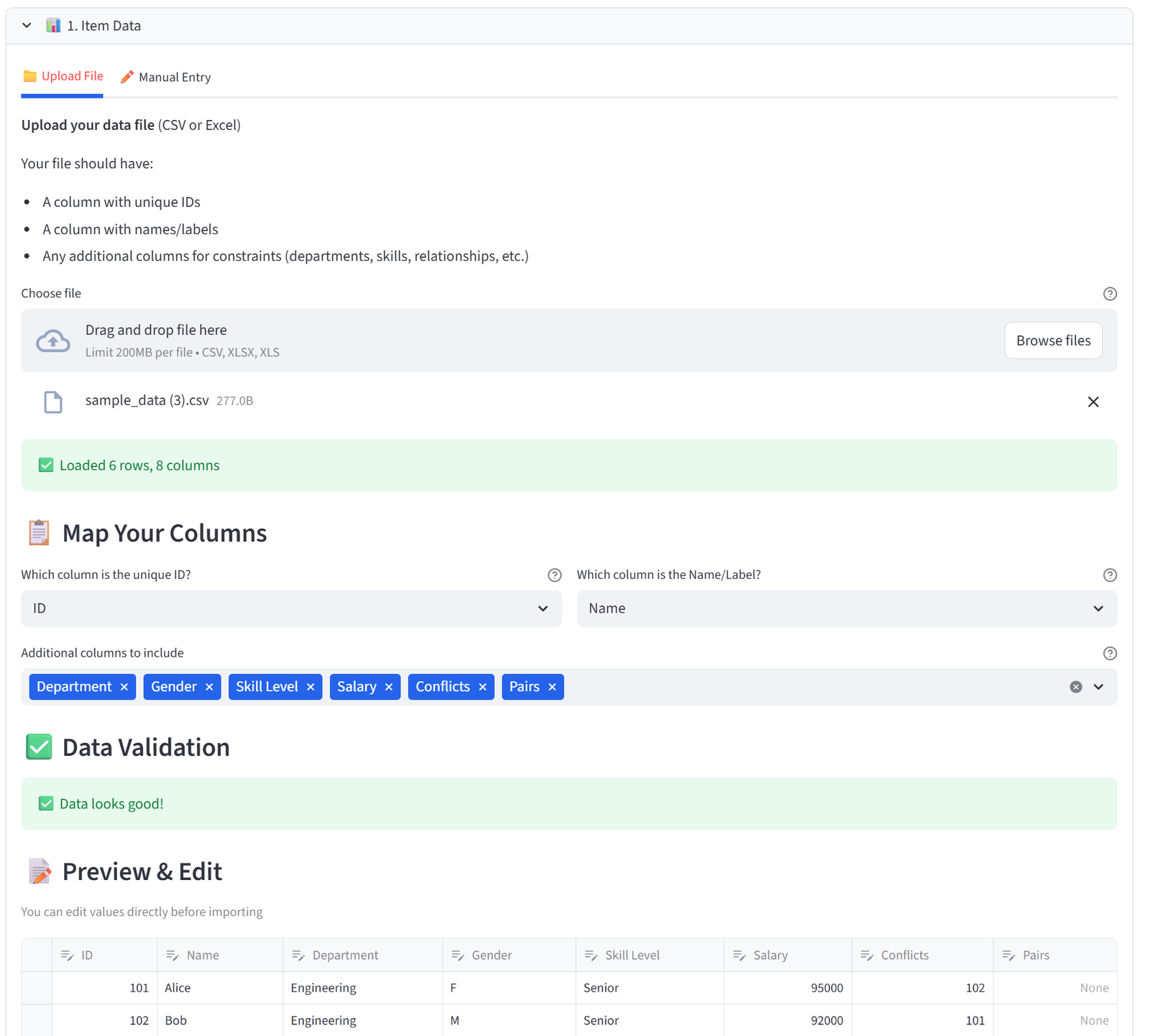
Step 2: Upload Your Data

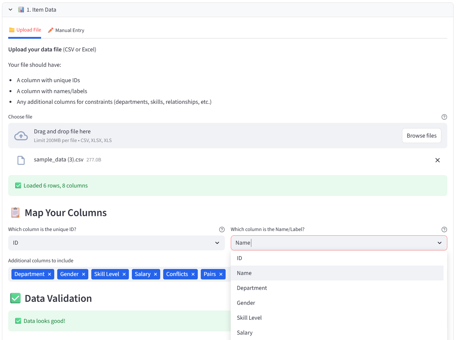
In the main area, use the file uploader under 1. Your Data to upload the CSV. The tool previews your data. Select the ID column and Name column using the dropdowns, then choose which columns to keep and click Import Data.

Step 3: Configure Groups

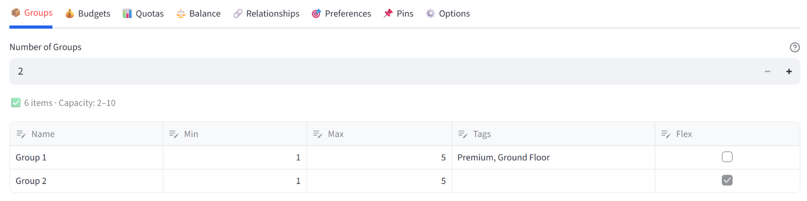
In the Configuration section, the Groups tab is selected by default. Set the number of groups (try 2). The tool auto-calculates min/max capacity. Rename the groups if you like.

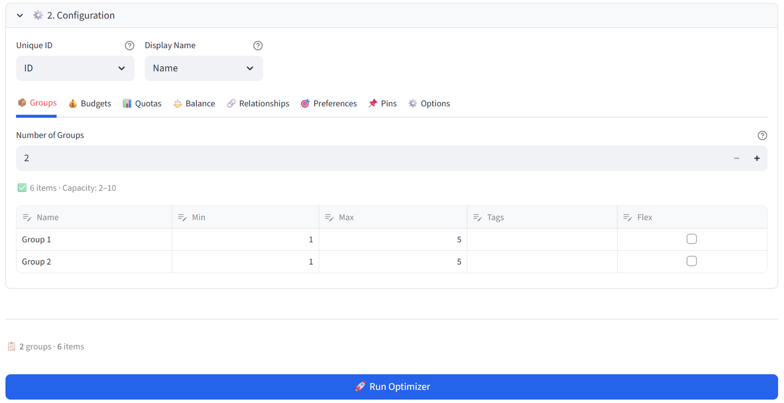
Step 4: Run the Optimiser

Scroll down and click the blue Run Optimizer button. Within seconds you will see a result summary and can explore the Overview, Rosters, Validation, Analytics, and Export tabs.

Step 5: Export Results

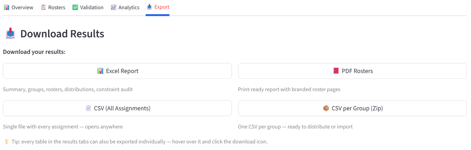
Go to the Export tab within Results. You have four download options:

Excel Report (.xlsx) — a fully formatted workbook containing a branded Summary sheet, a Group Summary with sizes and budget totals, a Constraints sheet listing every rule as an audit trail, an All Assignments sheet, one sheet per group, and distribution cross-tabulations for every categorical column. This is the most comprehensive export.
PDF Rosters — a print-ready branded report with one page per group showing the roster and summary statistics. Hand these directly to teachers, team managers, or shift supervisors.
CSV (All Assignments) — a single flat file with every item and its assigned group. Opens in any spreadsheet application. Use for importing into other systems.
CSV per Group (Zip) — a zip archive with one CSV per group, named after the group. Use when you need to email individual rosters to different people.

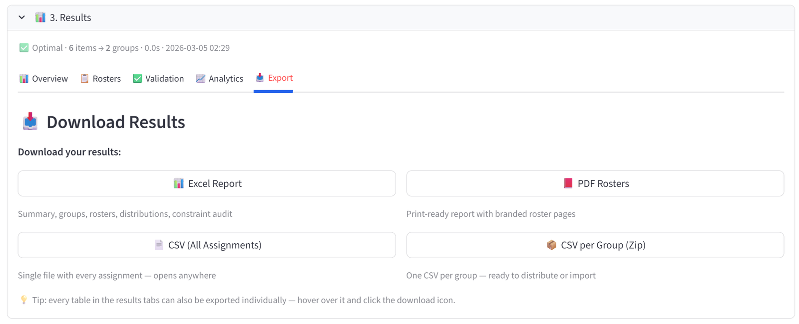
Every table elsewhere in the results tabs can also be exported individually — hover over any table and click the download icon in the top-right corner.

Getting Your Data In

Uploading a File

The tool accepts CSV and Excel (.xlsx) files. Your file needs at minimum a unique ID column. Additional columns are used by the constraint features.

File Requirements

One row per item
A unique identifier column (numbers or text)
Headers in the first row
No merged cells (for Excel files)

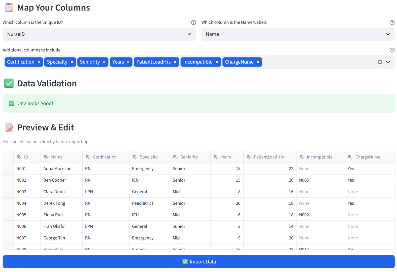
Column Mapping

After upload, you select which column is the Unique ID and which is the Display Name. These appear in the compact dropdowns at the top of the Configuration section. You can change them later in the Options tab.

Manual Entry

If you don’t have a file, you can build your dataset directly in the tool. Switch to the Manual Entry tab under “1. Your Data.” Type your column names as a comma-separated list — for example, Student ID, Name, Gender, Reading Level, IEP Hours — and click Create Table. You need at least two columns (an ID and a Name).

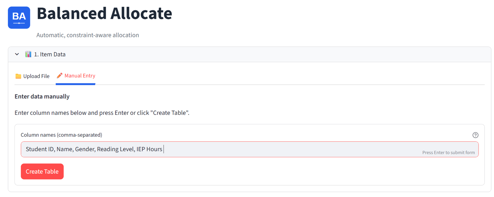
This creates an empty data editor where you can type values directly into cells. Click the + button at the bottom of the table to add new rows. Each row represents one item to be allocated. You can add as many rows as you need — the editor scrolls and supports hundreds of rows.

The default column suggestions (ID, Name, Department, Gender) are just placeholders. Replace them with whatever columns your scenario needs. The column names you enter here become available throughout the Configuration tabs for budgets, quotas, balance, relationships, and preferences.

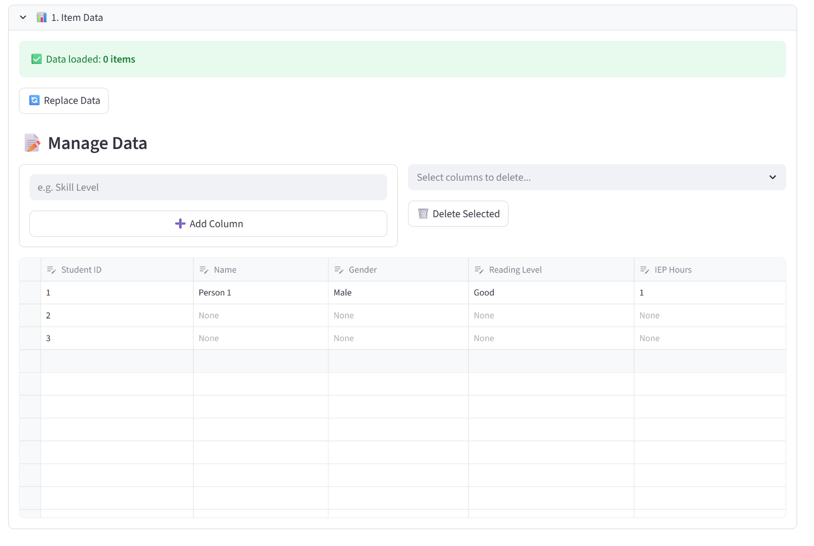
Managing Data After Import

Once data is loaded — whether uploaded or manually entered — the interface switches to a management view with several tools:

The data editor is a live, editable spreadsheet showing all your data. Click any cell to edit its value. Click the + button to add rows. Select a row and press Delete to remove it. The editor supports sorting by clicking column headers and resizing columns by dragging the header borders. Changes are held in the editor’s state and committed to the solver when you click Run Optimizer — you don’t need to save manually.

Add Column lets you add new columns to your dataset after import. Type a column name (e.g. “Skill Level”) and click the button. The new column appears in the editor with empty values for you to fill in. This is useful when you realise mid-setup that you need an extra attribute for a budget or quota rule.

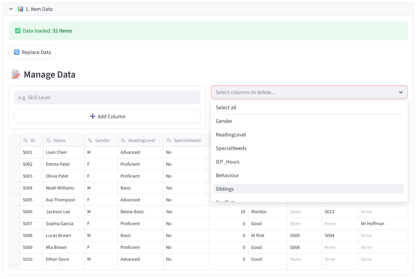
Delete Columns lets you remove columns you don’t need. Select one or more columns from the dropdown and click Delete Selected. The ID and Name columns cannot be deleted. Removing a column also removes it from any constraint that referenced it, so check your rules afterwards.

Replace Data clears the current dataset entirely and returns you to the upload/manual entry screen. This also resets all constraints, since the old rules may reference columns that no longer exist. If you want to keep your rules and just swap the data, use the Rules only save in the sidebar: save your rules first, replace the data, then load the rules back.

Every table in the data editor — and throughout the results — supports CSV export: hover over any table and click the download icon in the top-right corner.

Configuration — Every Tab Explained

All allocation rules live in the tabbed interface under 2. Configuration. The ID and Name column selectors sit at the top, followed by eight tabs.

Groups

Set the number of groups and configure each one.

Column	Purpose
Name	Display name for each group (rename freely)
Min	Minimum items this group must receive
Max	Maximum items this group can hold
Tags	Comma-separated labels for targeting in quotas/preferences (e.g. ‘Premium, Ground Floor’)
Flex	When ticked, capacity is soft — the solver can slightly exceed limits if it improves the result

A capacity summary line below the number input shows whether your total min/max range covers all items. Warnings appear if items exceed capacity.

Tip: Use Tags to create group categories. Then in Quotas or Preferences you can target ‘Tag: Premium’ to apply a rule to all tagged groups at once.

Budgets

Set min/max totals for any numeric column, per group. For example: max salary of $500K per team, or max weight of 1,200kg per truck.

How It Works

Select one or more numeric columns from the multiselect.
A table appears for each column with rows for every group.
Set Min Total and Max Total per group.

This is how you enforce resource limits. If you’re loading trucks, set max Weight per truck. If you’re forming teams, set a salary cap per team. If you’re placing tenants, set a revenue floor per building. The solver treats these as hard constraints — it will not produce a result that violates a budget limit.

If your budget limits are too tight for the data, the solver will report infeasibility and tell you which limits conflict. For example, if your total salary across all employees is $1.8M but you set max $400K per team across 4 teams ($1.6M total capacity), the solver will explain that the salary budget is impossible to satisfy.

You do not need to set both Min and Max. Leave Min at 0 if you only care about a ceiling. Leave Max at a very large number (e.g. 999999) if you only care about a floor. The solver only constrains what you explicitly set.

Combined Budgets

Sometimes you need a single limit across multiple groups. For example, two buildings sharing a total capacity. Use the Combined Budget section below the individual budgets to select a column, pick the groups to combine, and set one shared min/max.

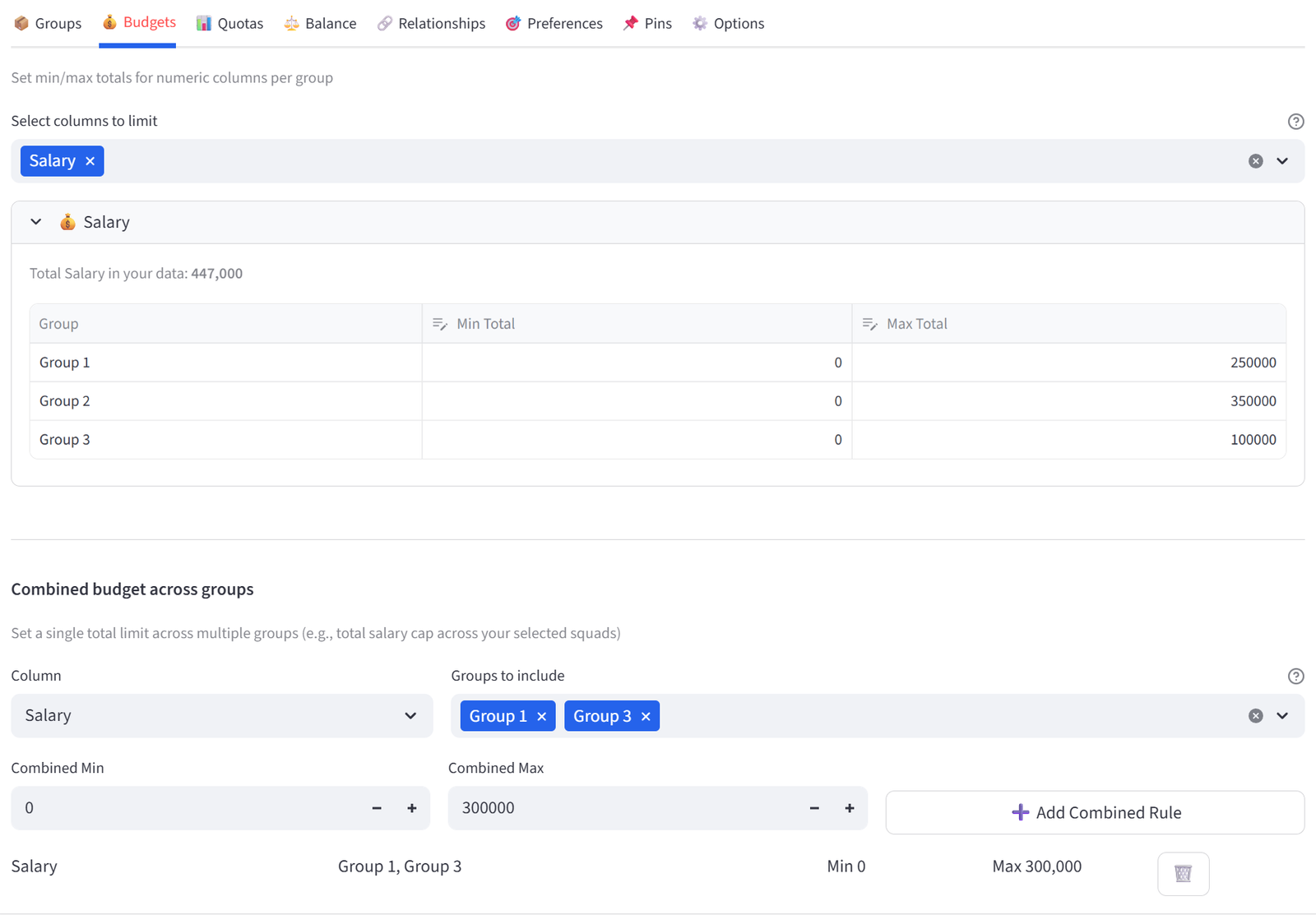
Tip: Combined budgets are ideal for shared resource pools where individual group limits are flexible, but the total is fixed. The solver can simultaneously consider both Individual Budget and Combined Budget limits to be adhered to. Set maximum Individual Budgets to a large value for any groups which should not be constrained.

Quotas

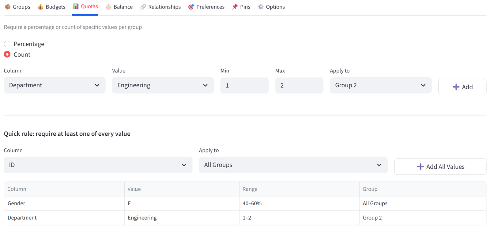
Require a percentage or count of specific values per group. For example: each team must be 40–60% female, or each shift must have at least 2 Charge Nurses.

How It Works

Toggle between **Percentage** and **Count** mode.
Select a column, a value to match, and the min/max range.
Choose which groups the quota applies to (All Groups, a specific group, or a Tag).
Click Add to create the rule.

Existing rules appear in a table below. Use the dropdown and delete button to remove rules.

A Quick Rule shortcut is available below the main quota form. Select a column and click “Add All Values” to create a count quota of Min 1 for every unique value in that column, applied to the group scope you select. This is useful when you want to guarantee at least one of every department, position, certification, or category in each group without adding rules one by one.

For example, selecting Position with Apply to All Groups creates a rule for each position (GS, GA, WA, C, WD, GD, GK) requiring at least 1 in every group. This is faster than adding 7 individual quota rules.

Note: Percentage quotas are calculated as a fraction of each group’s actual size, not of total items.

Balance

Control how attributes are distributed across groups. Three modes are available:

Mode	What It Does	Example
Equal	Spreads each unique value evenly across groups	Every team gets roughly the same number of Engineers
Maximise	Concentrates high values in target group(s)	Push top scorers into the A-team
Minimise	Concentrates low values in target group(s)	Put the lightest packages in the small van

Equal mode works with categorical columns (text values). Maximise and Minimise work with numeric columns and require you to select one or more target groups.

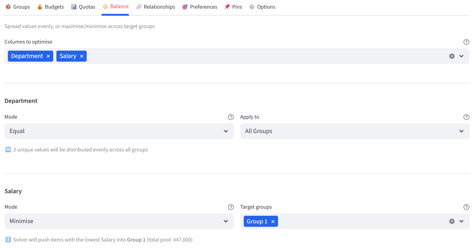
Tip: Maximise and Minimise now support multi-group targeting. Select multiple groups to concentrate values across all of them.

Balance is one of the most powerful features because it controls distribution without requiring you to know the exact numbers. Equal mode on a Department column means “spread departments evenly” — you don’t need to calculate how many Engineers should be in each team. The solver does that for you based on the data and group sizes. If you have 20 Engineers across 5 teams, it will aim for 4 per team. If you have 22, it will put 4 in some and 5 in others, as evenly as possible.

For the select/reject pattern (e.g. scholarship selection), Maximise is how you tell the solver “pick the best.” Set Maximise on MeritScore targeting the Awarded group, and the solver will select the highest-scoring applicants that satisfy all other constraints. The reject group gets whatever is left.

For asymmetric grading (e.g. netball teams), you can combine Maximise on the strong team with Preferences steering weak players to the development team, and Budget bands locking the middle teams together. This three-layer approach creates non-uniform distributions that would be nearly impossible to calculate manually.

Maximise and Minimise only work on numeric columns. They sum the column values in the target group and try to make that sum as high (or low) as possible. If your column has text values (like hazard class labels), you need to add a numeric equivalent column. For example, add a HazScore column where “None” = 0, “Class 3” = 3, etc.

Relationships

Define which items should be together or apart based on ID references in your data.

Type	Meaning
KEEP_APART	These items must NOT be in the same group (e.g. conflicts, rivals, exes)
KEEP_TOGETHER	These items SHOULD be in the same group (e.g. siblings, couples, partners)

How It Works

Your data must have a column containing IDs of related items, separated by a delimiter (default: semicolon). For example, if student S001 has a Conflicts column value of ‘S015’, the solver will keep S001 and S015 in different groups.

Select the column containing related IDs.
Choose KEEP_APART or KEEP_TOGETHER.
Set the separator character.
Toggle Required (hard) or Preferred (soft).

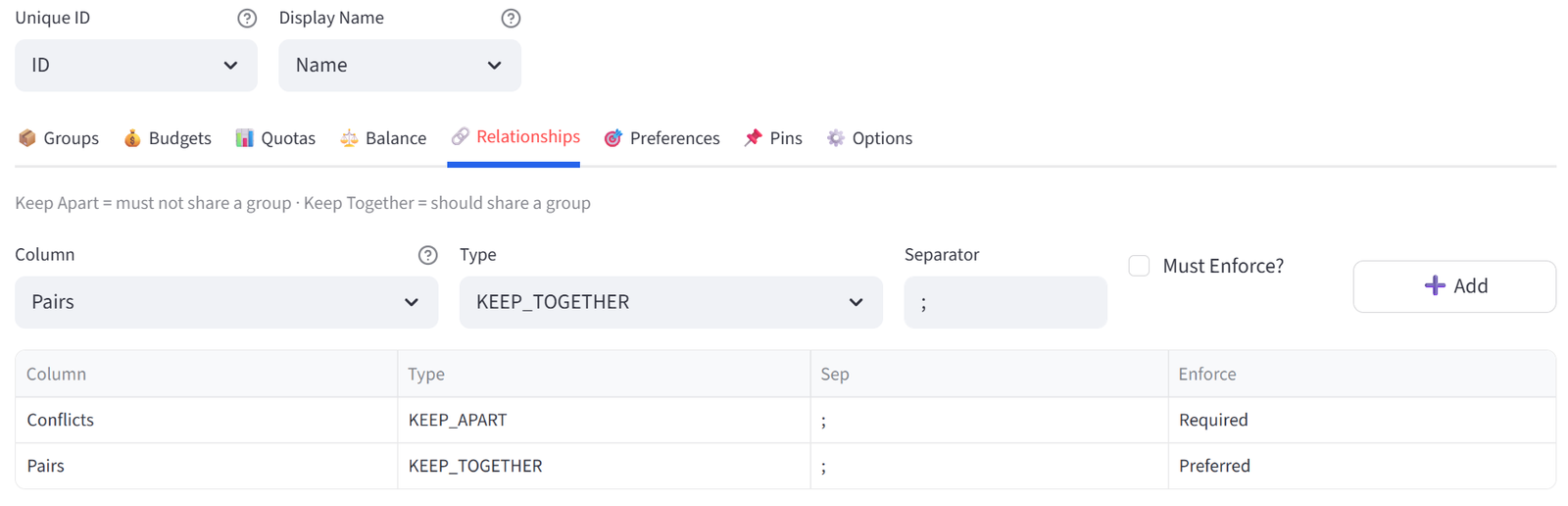
Note: Hard relationships (‘Must Enforce’ ticked) are enforced strictly. Soft relationships (‘Must Enforce’ not ticked) are preferred but can be broken if other hard constraints make it impossible.

Common issues with relationships:

The most frequent error is putting shared labels (like family surnames) in the relationship column instead of IDs. The column must contain the IDs of the related items, not a group label. For example, if Robert Taylor (G003) and Linda Taylor (G004) should sit together, G003’s Family column should contain “G004” and G004’s should contain “G003” — not “Taylor” in both. The solver matches on IDs, not labels.

If you have multiple related items, separate them with the delimiter character (default semicolon). For example, if a student conflicts with three others: “S015;S020;S028”.

Relationships are bidirectional in effect but only need to be declared in one direction. If G003 lists G004 as a family member, the solver keeps them together regardless of whether G004 also lists G003. However, listing in both directions is good practice for clarity and won’t cause issues.

If the tool warns that relationship IDs are not found in your data, check for whitespace, case sensitivity, or float formatting (e.g. “101.0” vs “101”). The tool normalises IDs on import, but if you added relationship values manually after import, they may not match.

Preferences

Express soft or hard preferences for where items should go, based on column values.

How It Works

Preferences let you say ‘items matching this condition should go to this group.’ You can match on exact values (Department = Engineering) or numeric thresholds (Salary > 100000).

Operator: = for exact match, >, <, >=, <= for numeric comparisons
Target: which group to prefer
Strength: 1–100, where higher means stronger preference. Or toggle Must for a hard constraint.

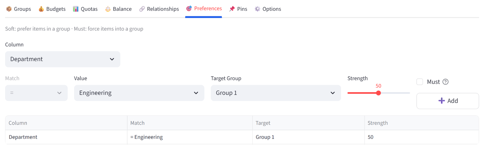
Tip: A preference with Must ticked becomes a hard constraint — the item MUST go to that group. Use this sparingly as it reduces solver flexibility.

Preferences vs Pins: Preferences are different from Pins in an important way. A Pin is absolute — the item must or must not go to a specific group, and the solver fails if it can’t honour it. A Preference is weighted — the solver tries to honour it but can override it if other constraints are more important. Use Preferences when you have a desired outcome but want the solver to have flexibility. Use Pins only when the assignment is non-negotiable.

How Strength interacts with Priority Sliders: The Strength value (1–100) on each preference controls its importance relative to other preferences. The Priority Slider for Preferences in the Options tab scales all preferences globally. So a preference at Strength 80 with the Preferences priority at 60% behaves differently than the same preference with the priority at 100%. If preferences aren’t being honoured, try increasing the Preferences priority slider before increasing individual strengths.

Numeric operator preferences are particularly useful for steering items by threshold. For example, “SkillRating < 55 → Rubies (Strength 85)” pushes low-rated players toward the development team without hard-pinning them. Combined with Maximise on the strong team, this creates the asymmetric grading pattern used in the Netball example.

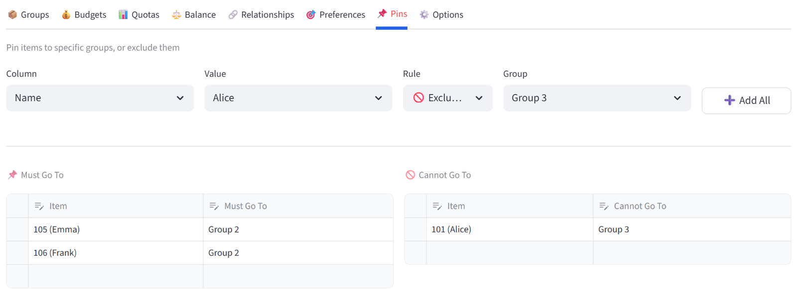
Pins & Exclusions

Force specific items into or out of specific groups. This is the most direct form of control.

Bulk Assign

Use the bulk assign row at the top to pin or exclude all items matching a column value at once. For example: pin all items where BridalParty is not empty to Table 1.

Manual Pins

The two side-by-side editors let you add individual pins and exclusions. Select an item and a group from the dropdowns. Use the + button to add rows.

Options

Fine-tune the solver and configure output.

Priority Sliders

When soft constraints compete, priority sliders control which ones the solver tries hardest to satisfy:

Slider	Default	What It Controls
Keep Apart	100	How important is it to separate conflicting items
Keep Together	80	How important is it to keep paired items together
Preferences	60	How strongly to honour preferred assignments
Balance	20	How important is even distribution of attributes

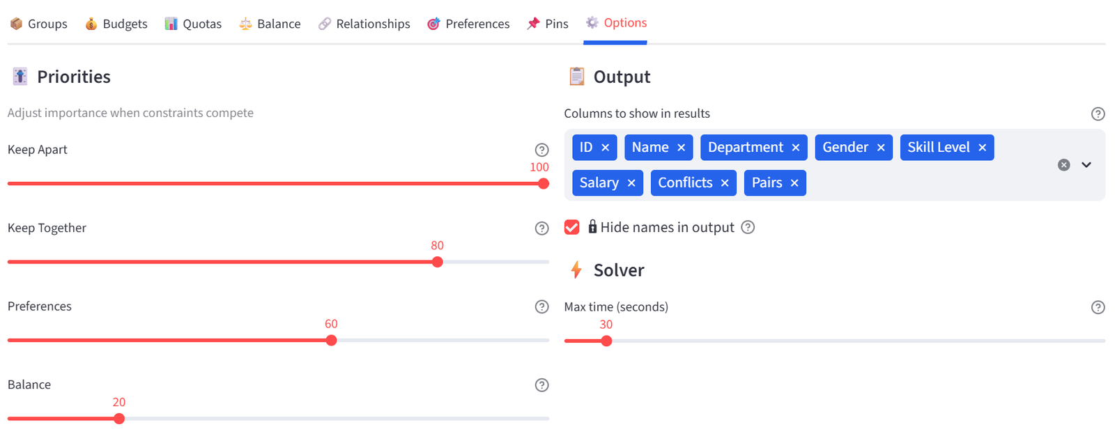
Output Options

Columns to show: select which columns appear in results.
Solver timeout: how many seconds before the solver stops (default 30). Increase for large or complex problems.
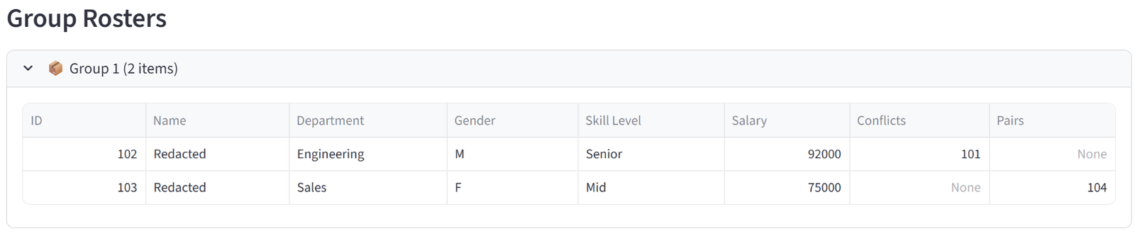
Hide names in output: will report the unique identifier (ID), but show the display name as ‘Redacted’ per below.
Lock solution prevents accidental re-runs. Once you’re happy with a result, tick this to disable the Run button until you untick it. This is useful when presenting results to stakeholders or when you’ve finished an allocation and want to ensure nobody accidentally overwrites it during an export or review session.

Running the Optimiser

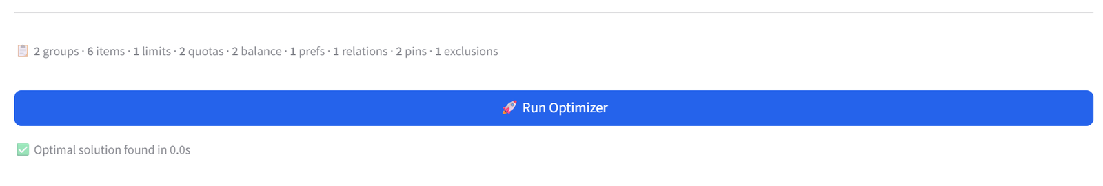
Constraint Summary

Below the Configuration section, a compact summary line shows your active constraints. For example: 6 groups · 700 items · 2 limits · 9 quotas · 1 balance. Only non-zero counts appear. This can be used as a sense-check to confirm the intended rules have been included and registering correctly (e.g. ‘Add’ button has been used where applicable).

Pre-Run Validation

The tool checks for common issues before running: capacity mismatches, empty data, invalid IDs in relationships. Any errors appear in red and prevent the solver from running.

Solution Status

Status	Meaning
Optimal	The mathematically best solution was found
Good (Feasible)	A valid solution was found within the time limit, though a better one may exist
Infeasible	No solution satisfies all hard constraints — see conflict report

Troubleshooting Infeasibility

If the solver reports no solution possible, a conflict report appears listing which constraints conflict. Common causes:

Total capacity (sum of group Max values) is less than the number of items
Hard quotas that are mathematically impossible (e.g. 50% of 5 items = 2.5)
Contradictory pins (item pinned to Group A but also excluded from Group A)
Too many hard constraints leaving no valid configuration

Tip: Start with fewer hard constraints. Use the conflict report to identify which constraint to relax. Switch hard rules to soft where possible.

Understanding Your Results

After a successful run, a compact summary line appears: status, items allocated, groups, solve time, and timestamp. Results are organised in five tabs.

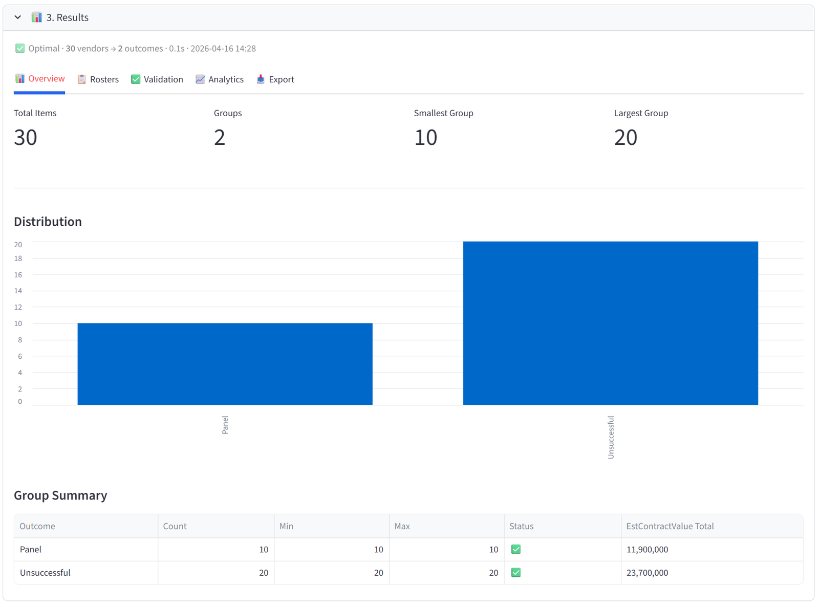
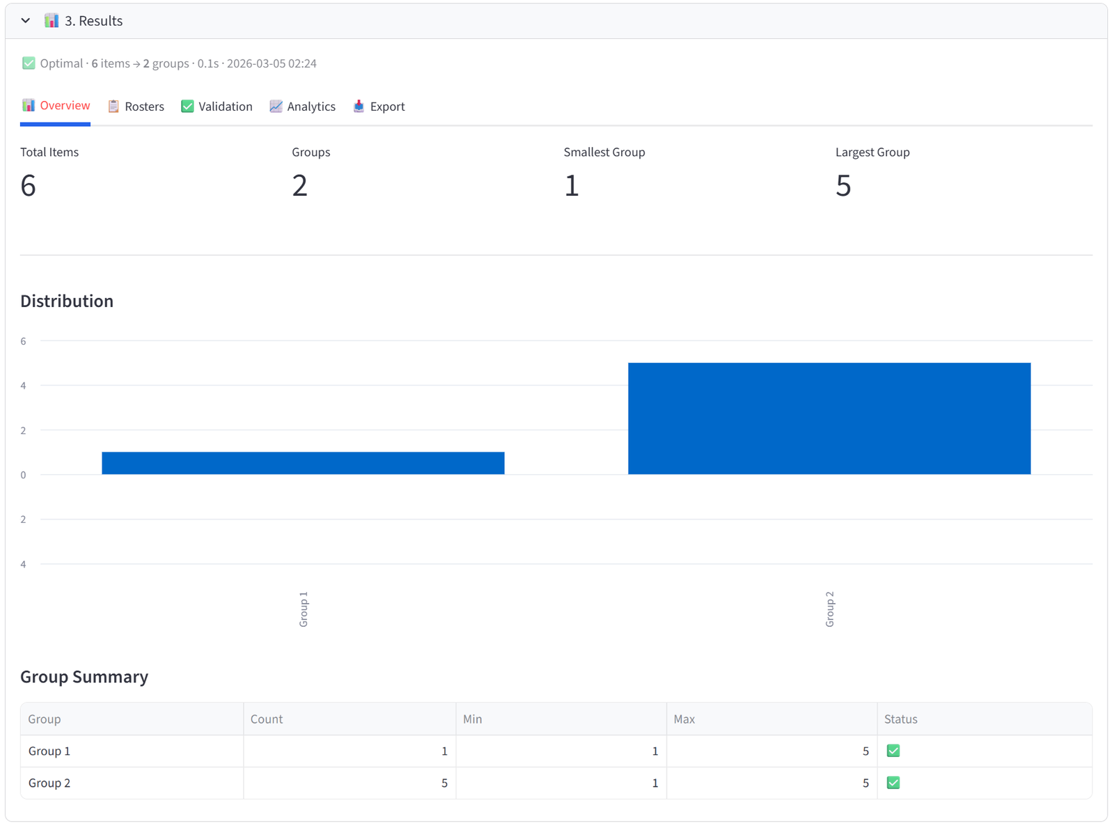
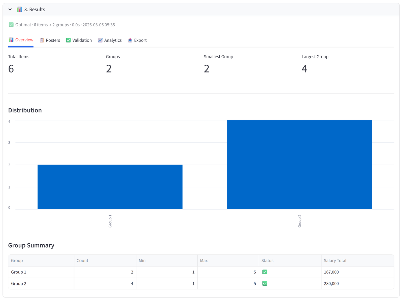
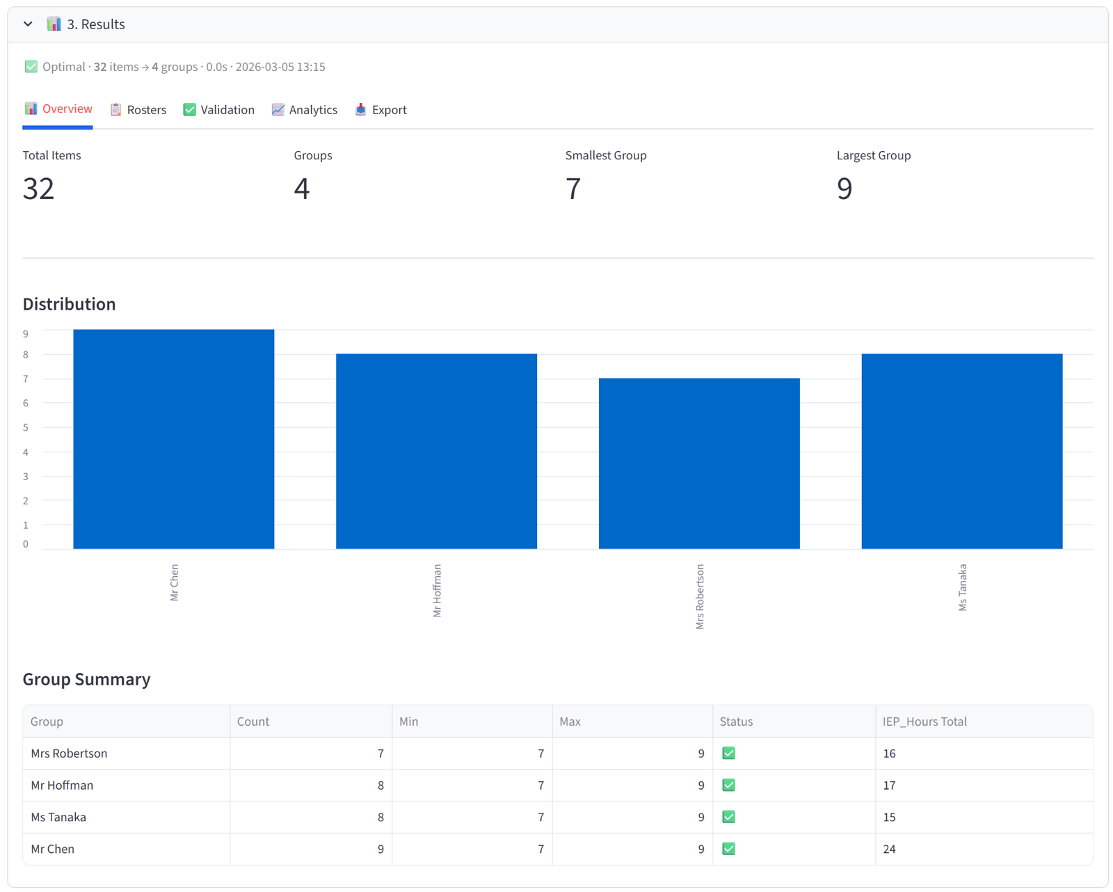
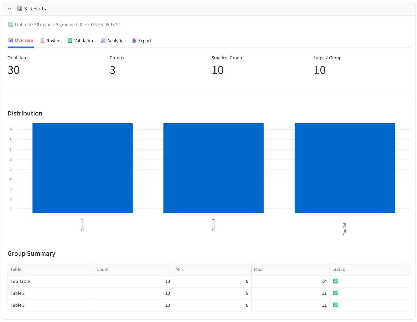
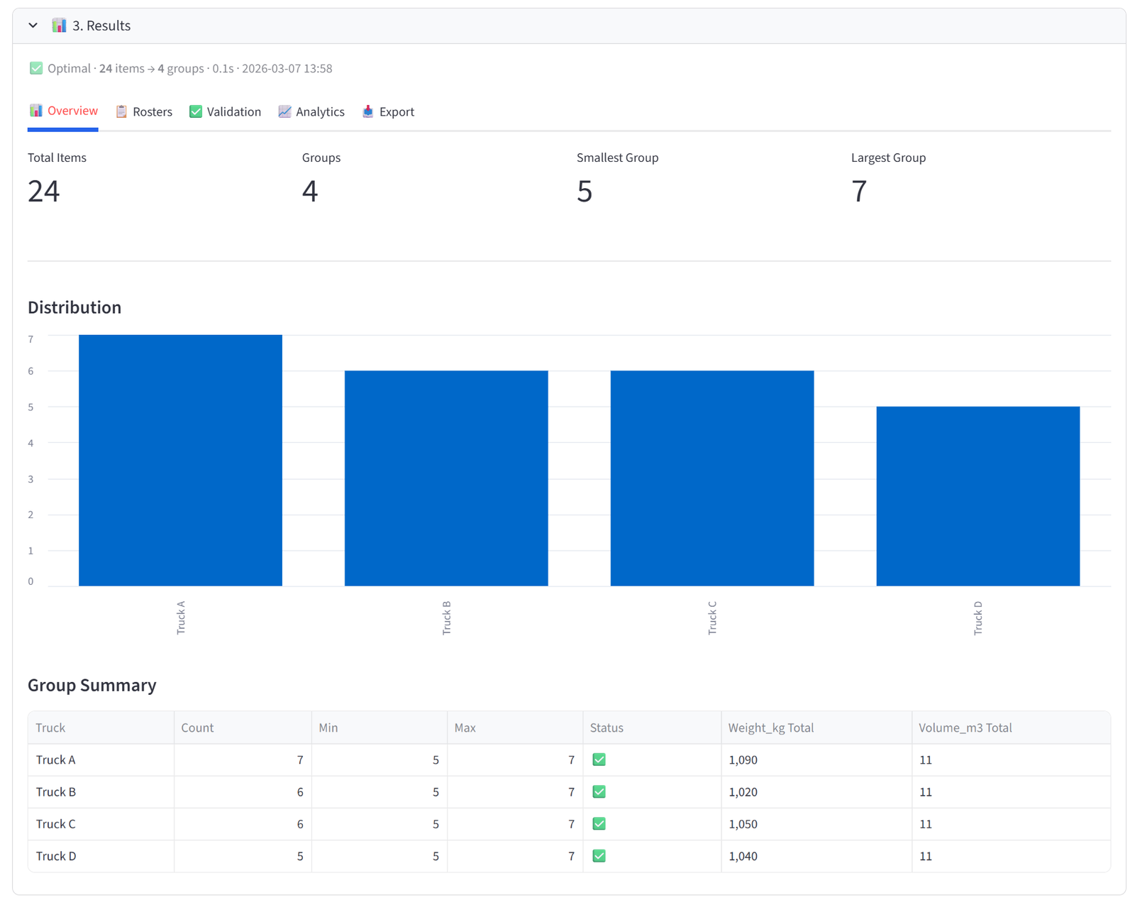
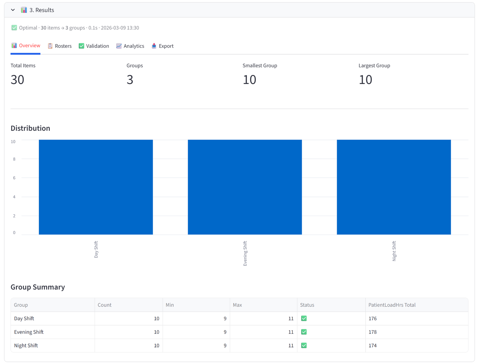
Overview

The Overview tab gives you an at-a-glance health check of the allocation. Four metrics appear at the top: Total Items, Groups, Smallest Group, and Largest Group. Below that, a bar chart shows the distribution of items across groups — any obvious imbalance is immediately visible.

The Group Summary table is the most useful element. Each row shows one group with its item count, min/max capacity, and a pass/fail status. If you set budgets, the table automatically appends columns showing the actual total of each budget column per group — so you can see at a glance that Team Alpha has $487,000 in salary, Team Beta has $462,000, and so on.

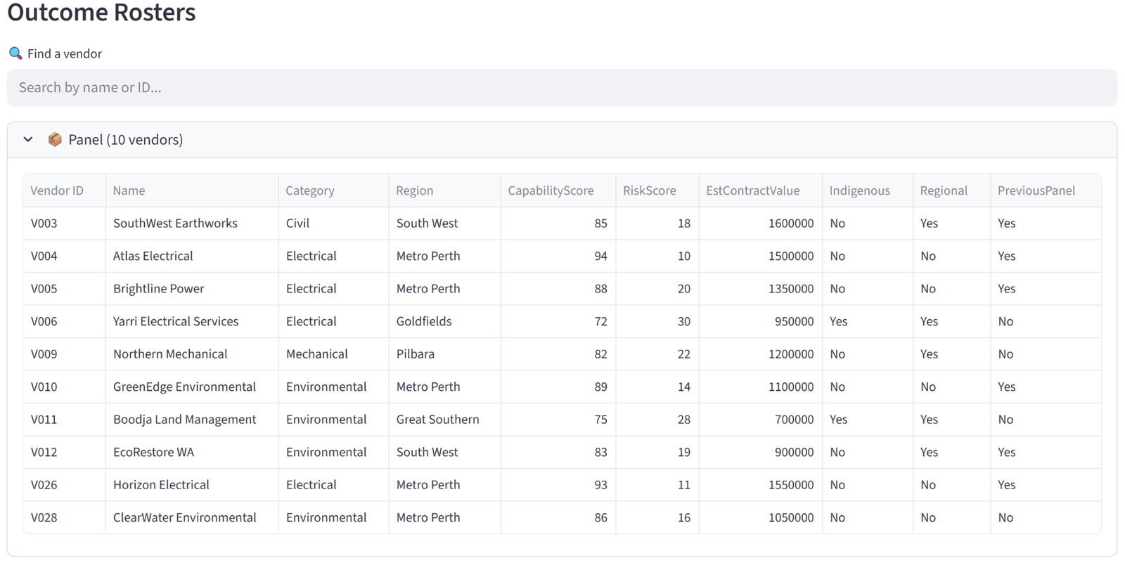
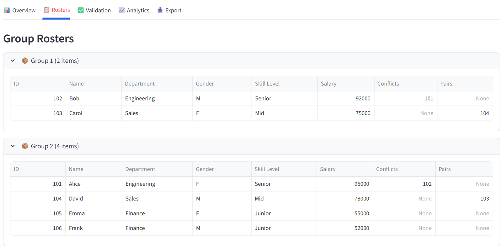
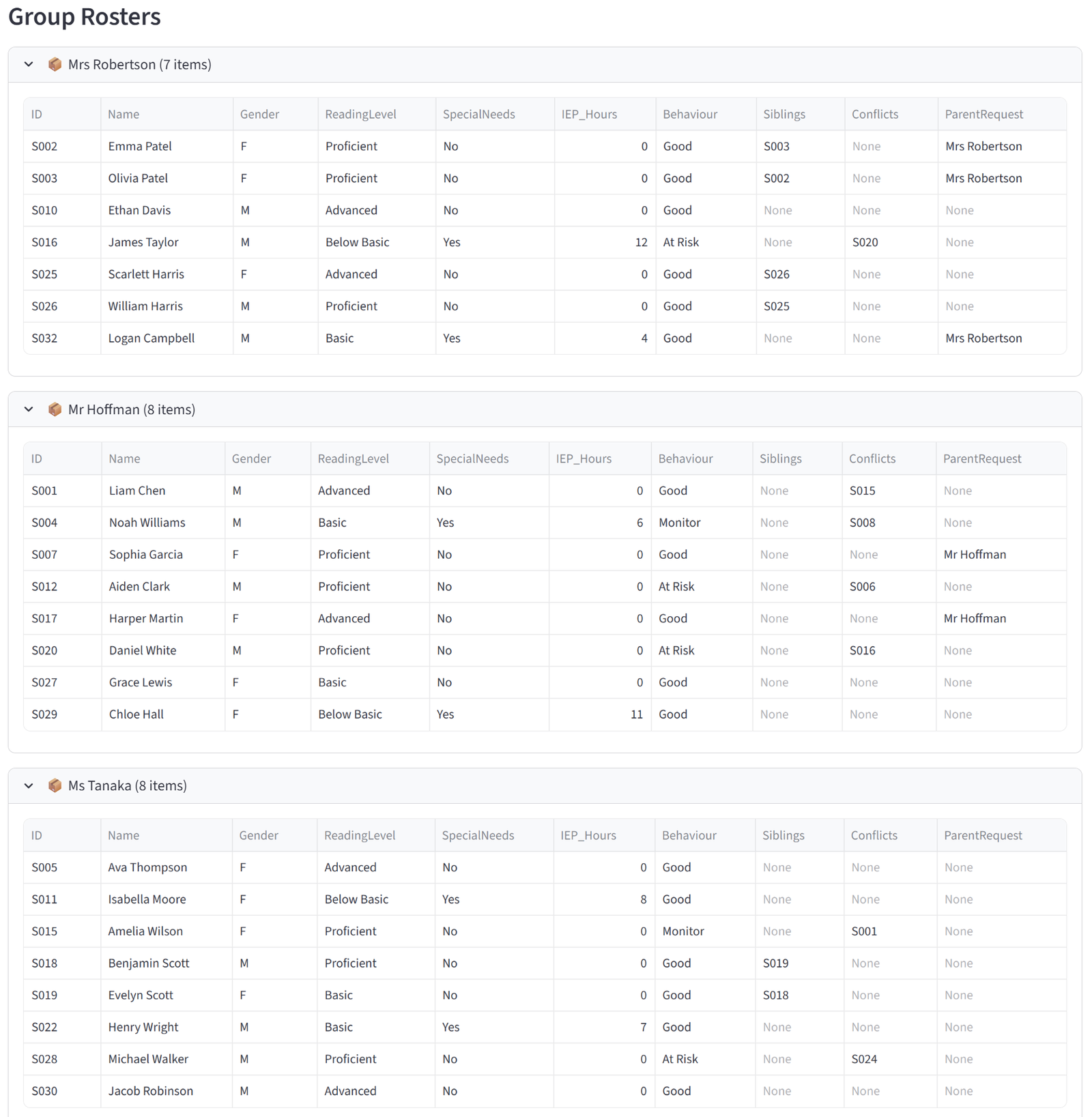
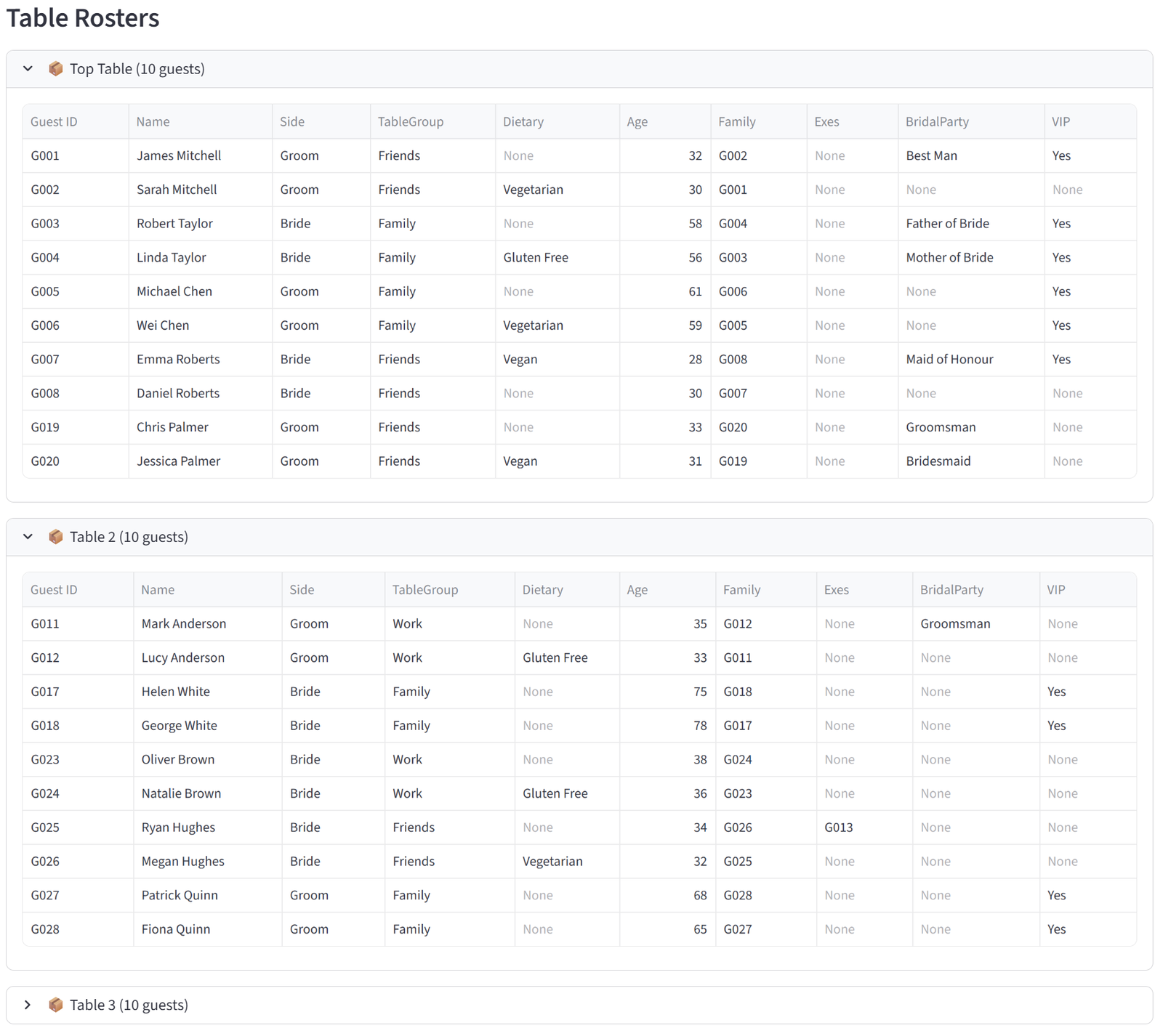
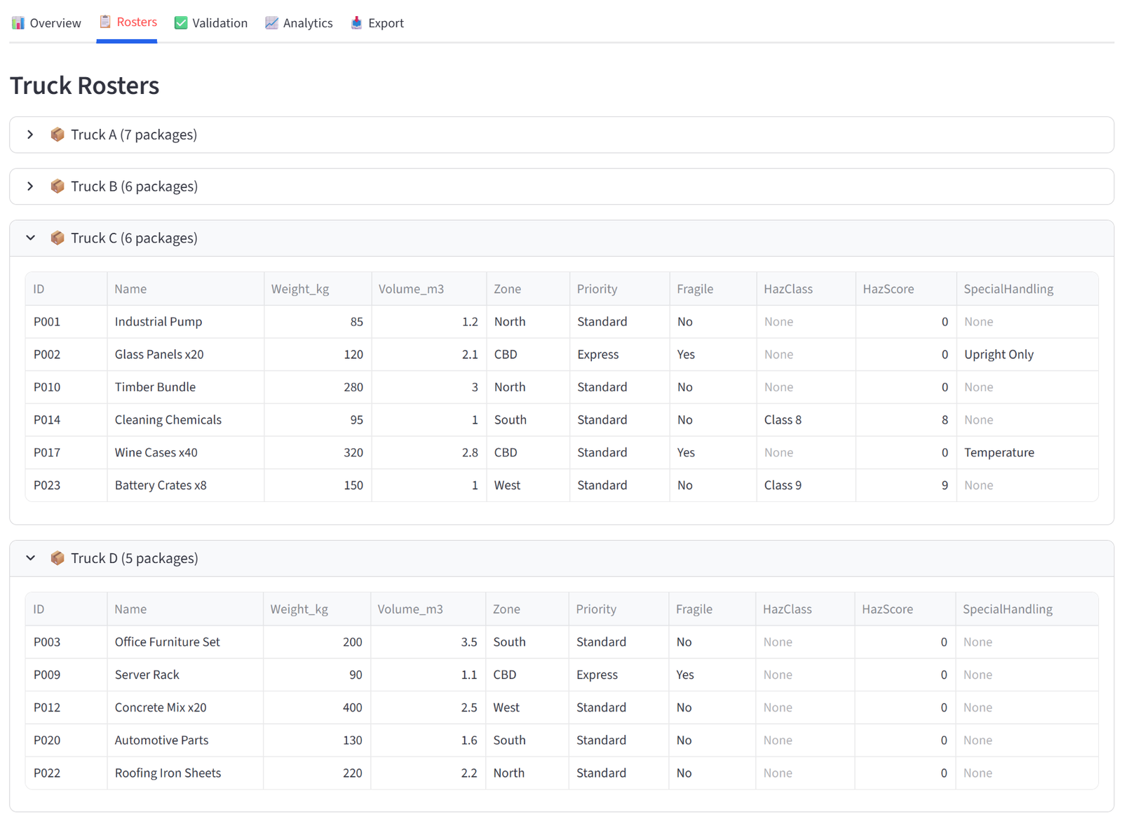
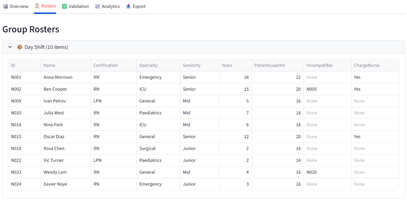
Rosters

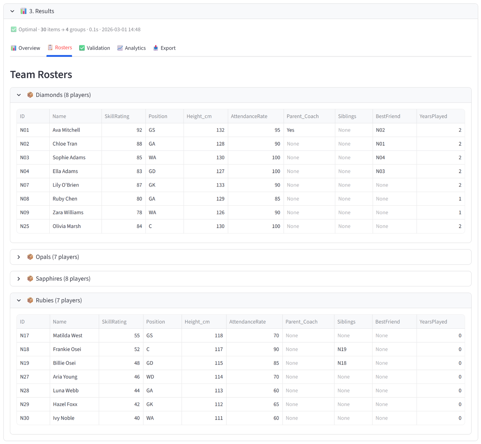
The Rosters tab shows one expandable panel per group, each containing a full data table of every item assigned to that group. The columns displayed are controlled by the “Columns to show” setting in the Options tab — you choose which columns matter for the final output. Each panel shows the group name and item count in its header.

These tables are what you would print, email, or hand out. A teacher gets their class list with student names, reading levels, and special needs flags. A logistics dispatcher gets their truck manifest with package weights and zones. A grading coordinator gets each team roster with player names, positions, and skill ratings.

Every table in the results — including these roster tables — supports individual export: hover over any table and click the download icon in the top-right corner to save it as a CSV. This means you can export individual group rosters without downloading the full report.

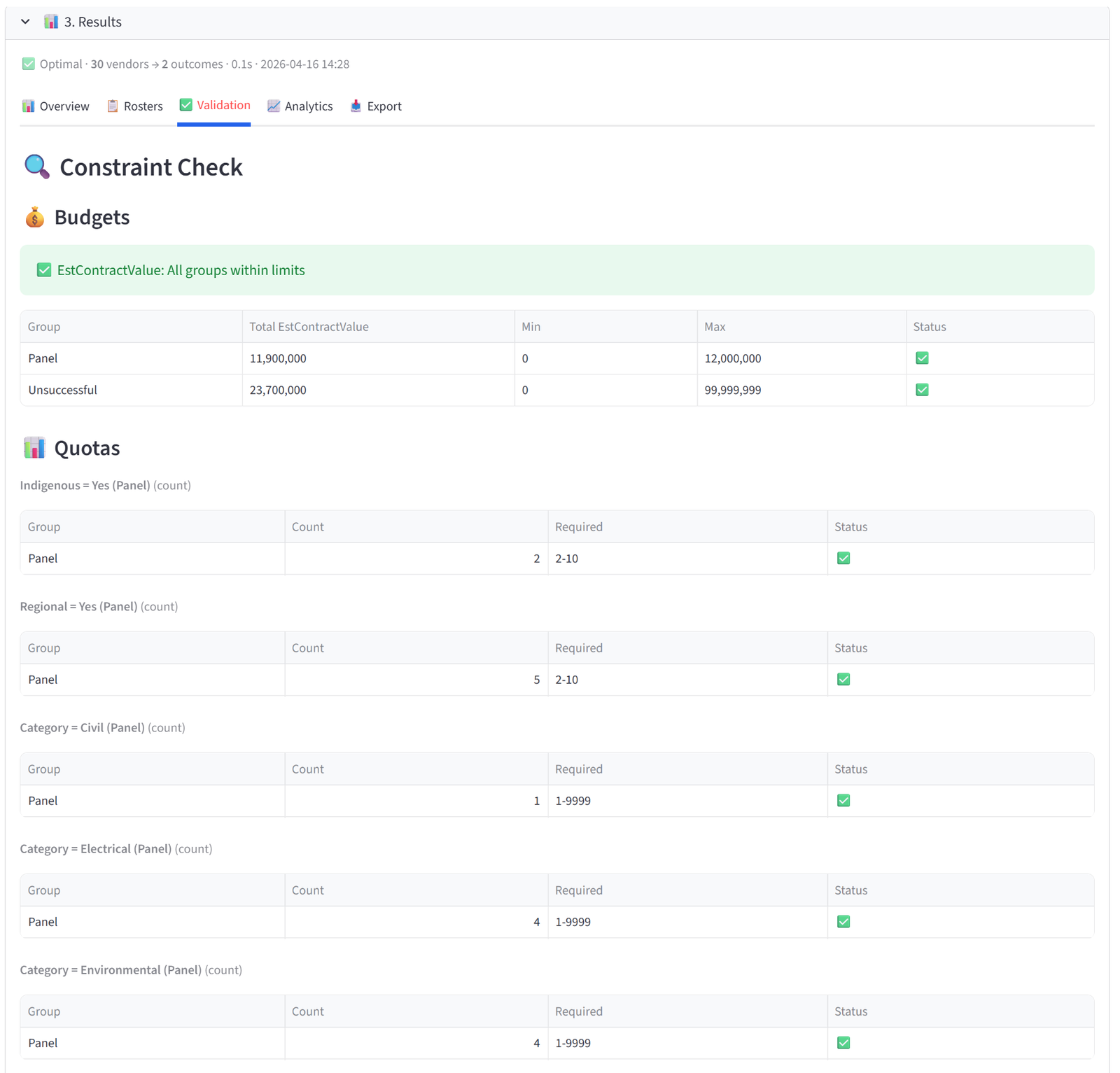
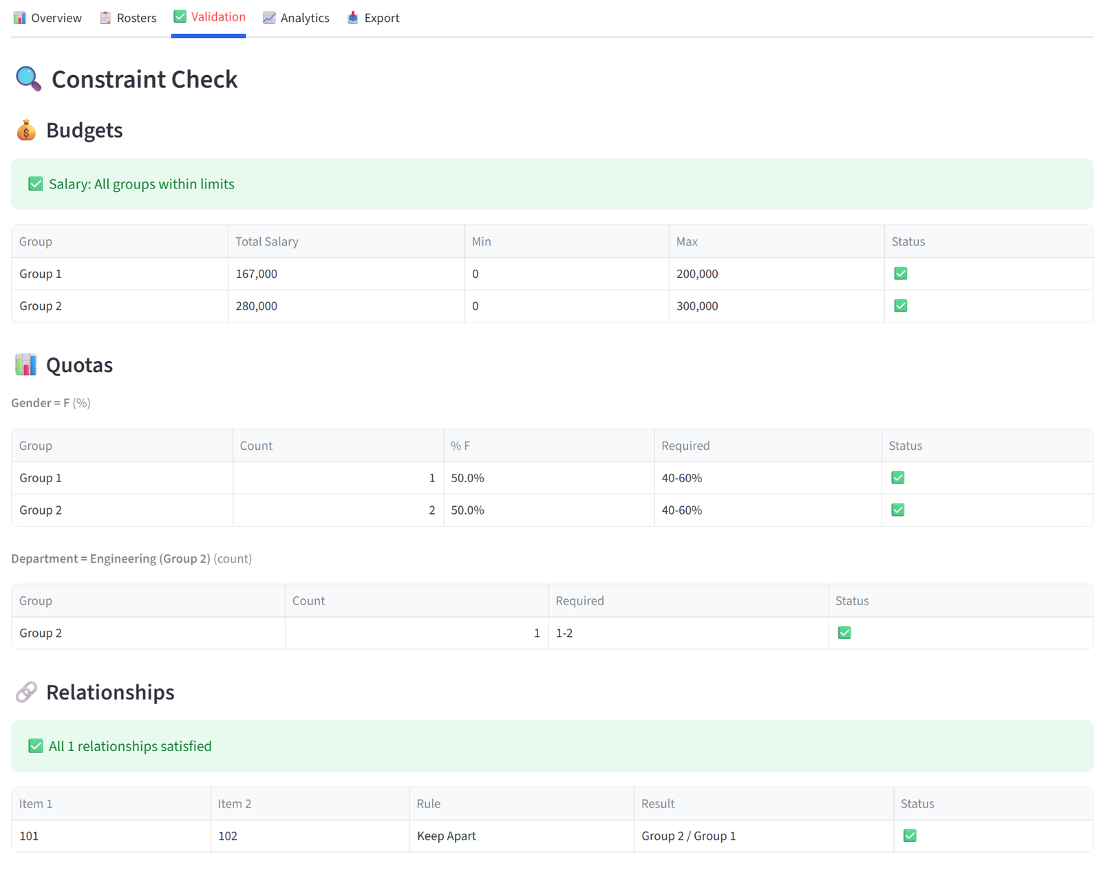
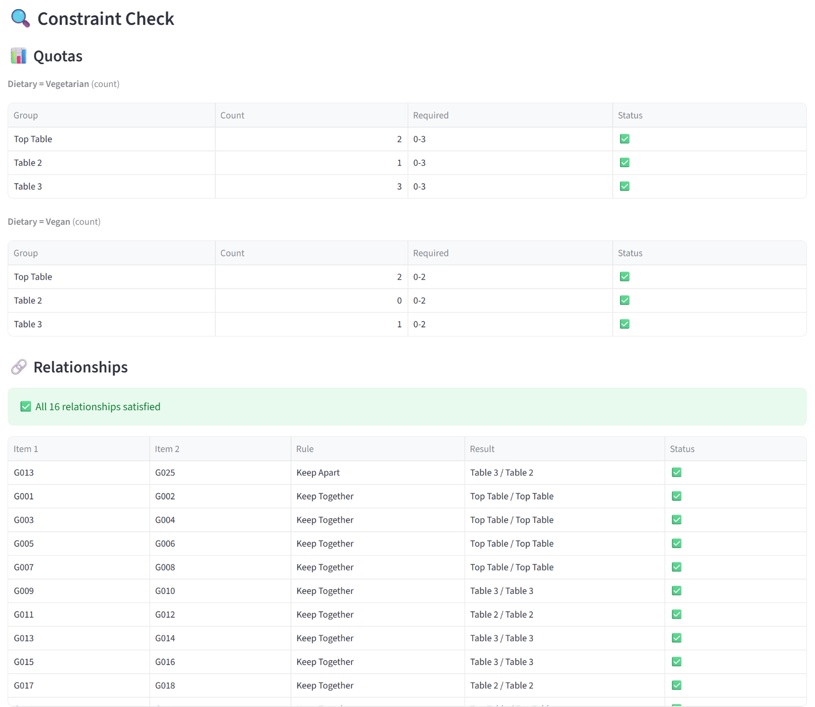
Validation

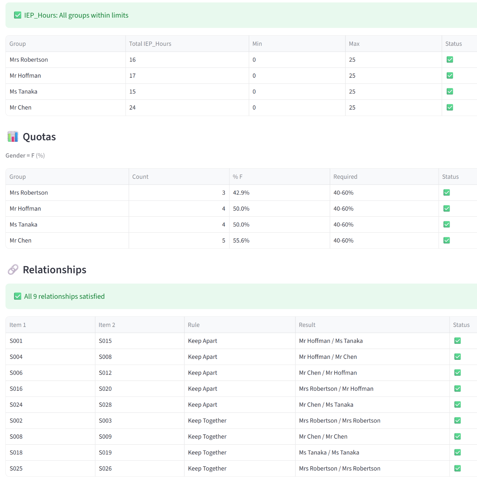
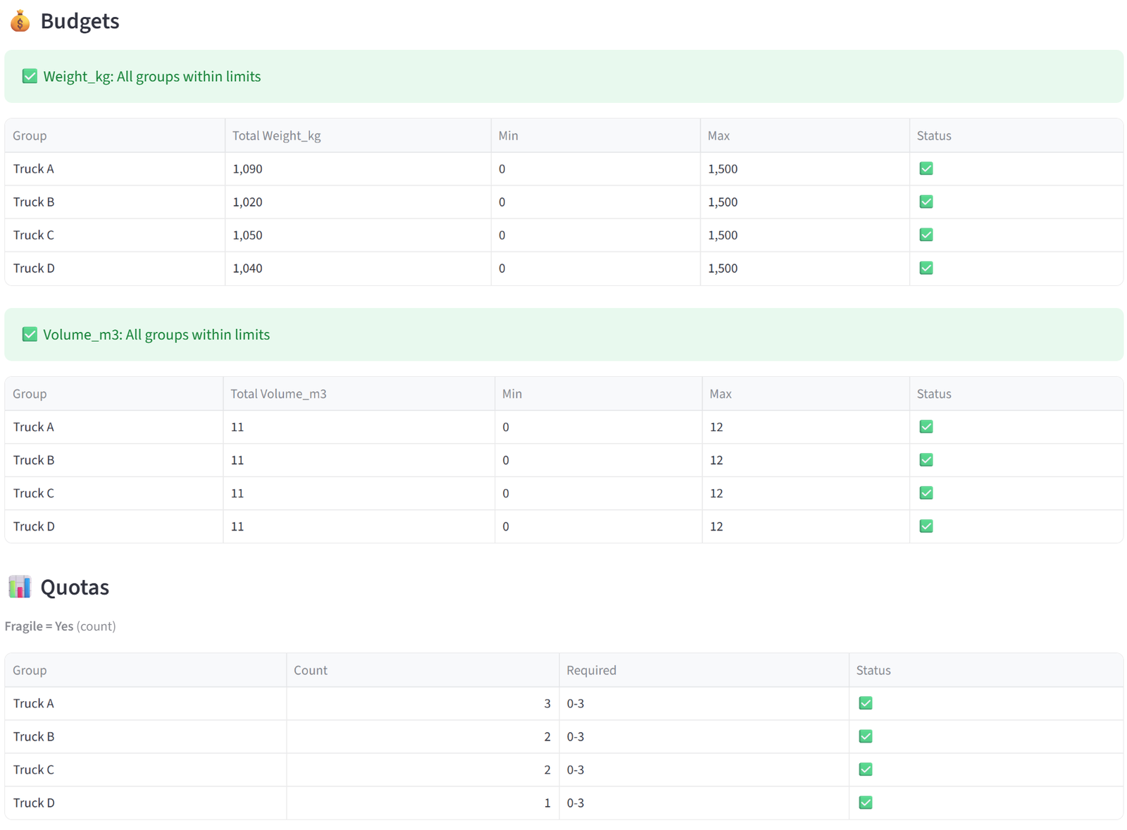
The Validation tab audits every constraint you set against the actual result. It is organised into sections by constraint type, and each section shows a detailed verification table with pass/fail indicators.

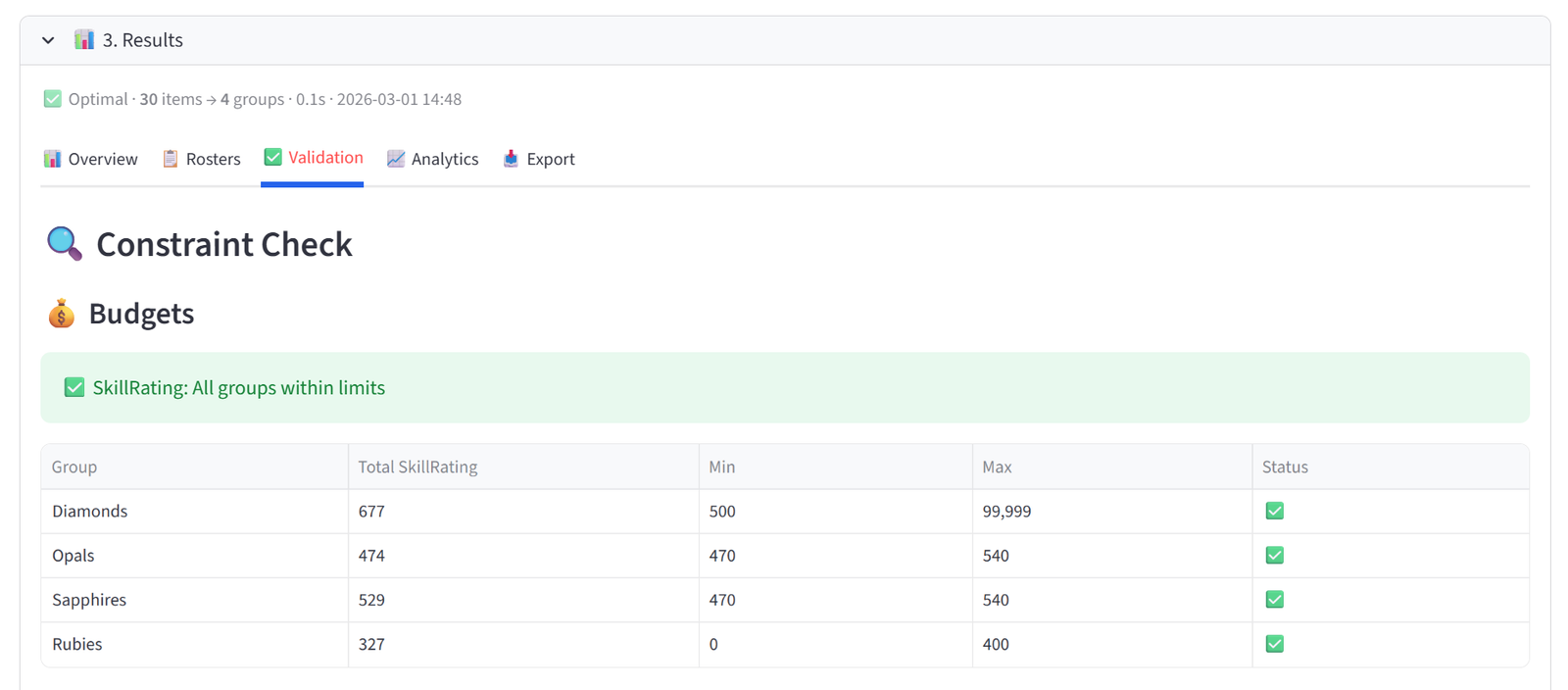
Budgets — for each budget column, a table shows every group’s actual total alongside the min/max you set, with a green tick or red cross. A summary line above confirms whether all groups are within limits or flags those that aren’t.
Combined Budgets — shows each combined constraint with the individual group contributions and the combined total, checked against your shared limit.
Quotas — for each quota rule, a table shows every targeted group with its actual count (and percentage, if in percentage mode) versus the required range. Quotas applied to specific groups or tags only show those groups.
Relationships — lists every relationship pair (keep-apart or keep-together) with the groups each item landed in and whether the rule was satisfied. Duplicate pairs are deduplicated. A summary line reports the total count and how many were violated.
Preferences — shows each preference rule with how many matching items landed in the target group versus how many matched overall, expressed as a count and percentage. Preferences are soft constraints, so partial satisfaction is expected and the tab notes this.
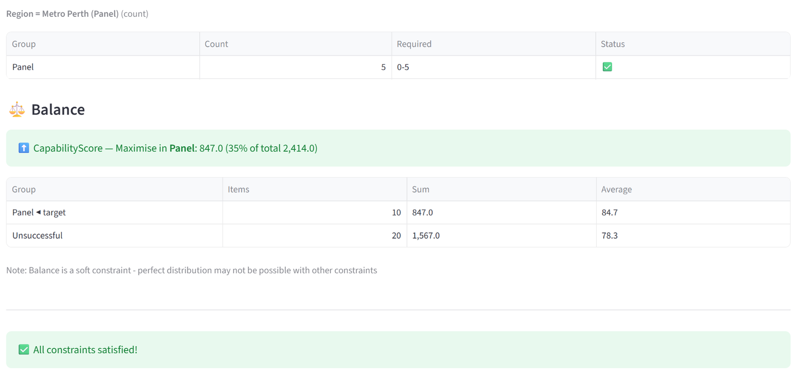
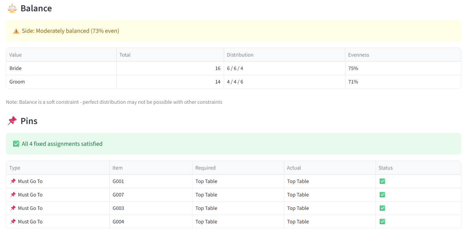
Balance — for Equal mode, shows a distribution table with each value’s count per group and an evenness percentage (100% = perfectly even). For Maximise or Minimise, shows the sum, count, and average per group with the target group marked, plus the percentage of total value concentrated in the target.
Pins & Exclusions — lists every pin and exclusion with the required group, the actual group, and pass/fail. Any violations are flagged in red.
At the bottom, a single summary line confirms whether all constraints passed or flags that some have issues.

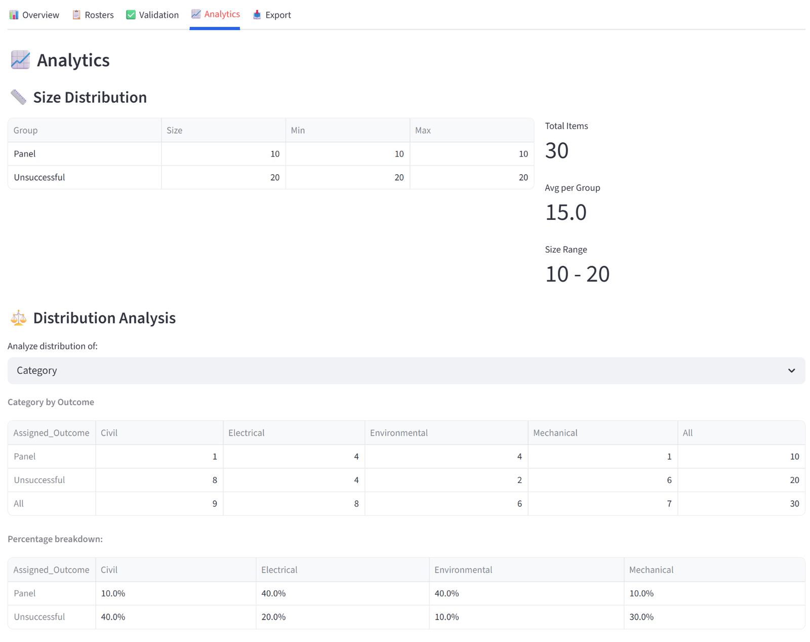
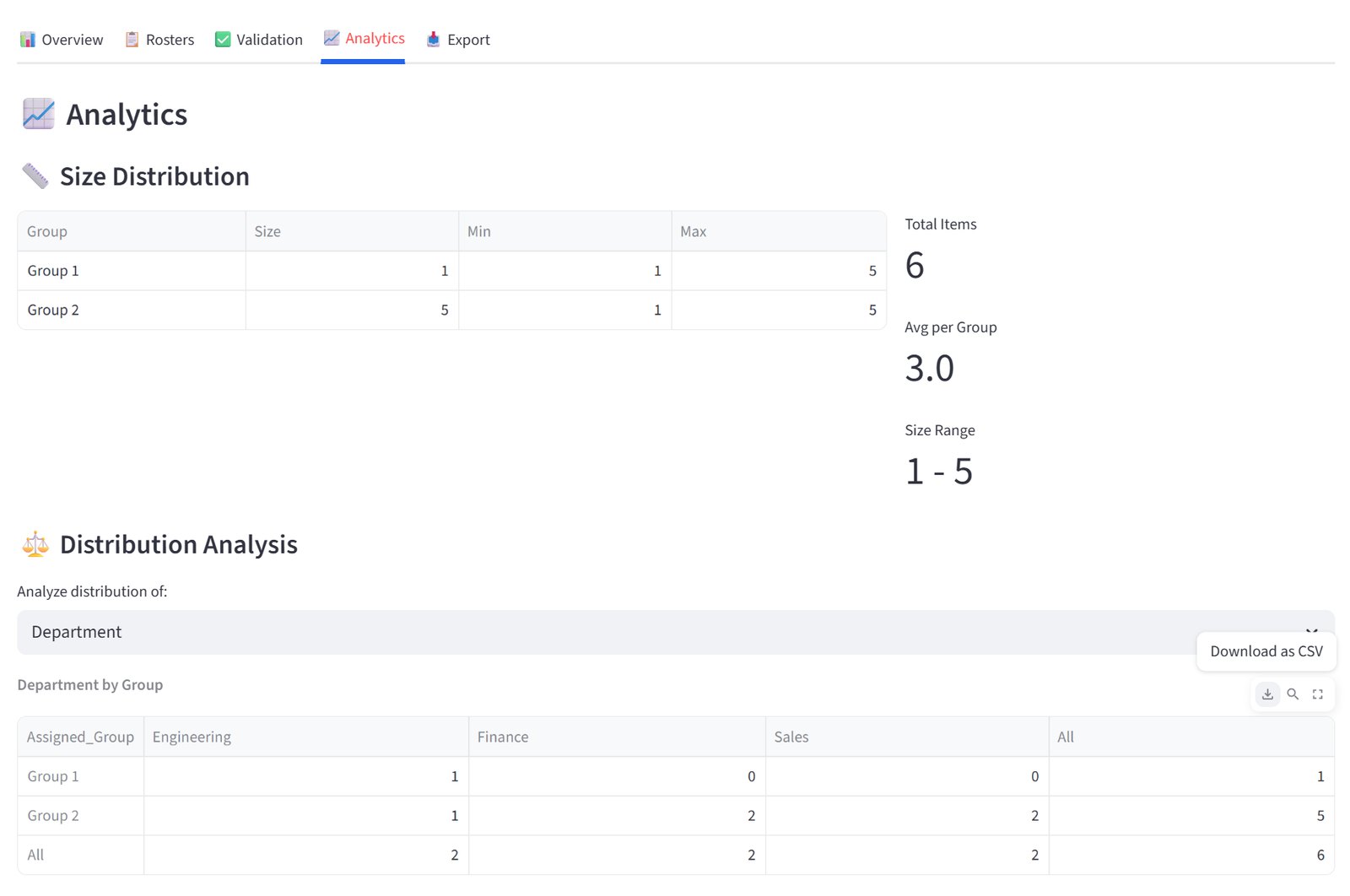
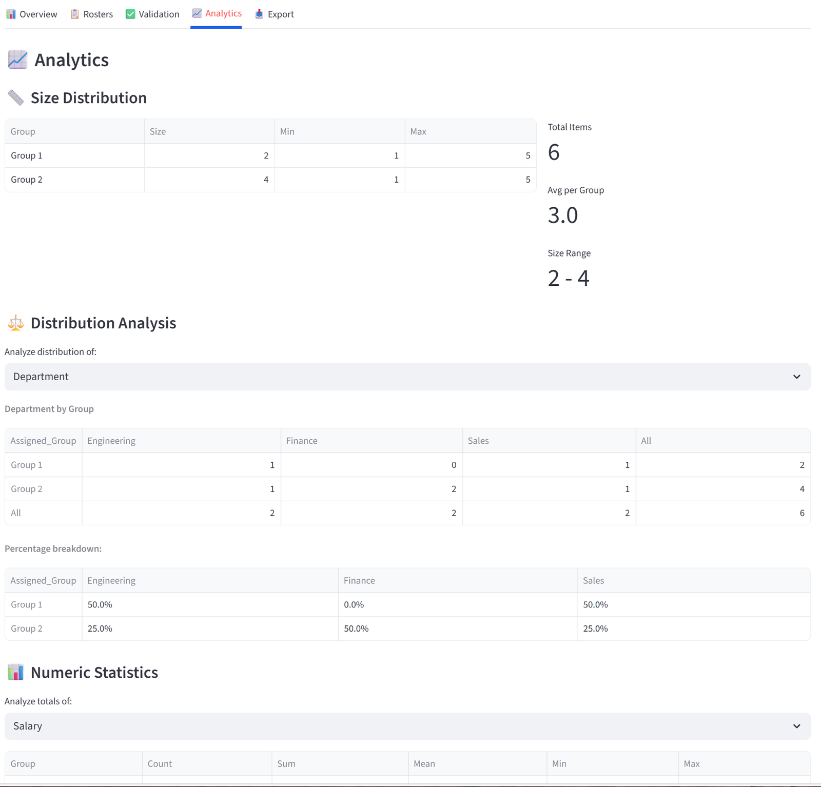
Analytics

The Analytics tab lets you explore the distribution of your data across groups interactively — not just for the columns you set constraints on, but for any column in your data via dropdowns.

Size Distribution shows a table of group sizes alongside capacity limits, plus summary metrics (total items, average per group, size range).
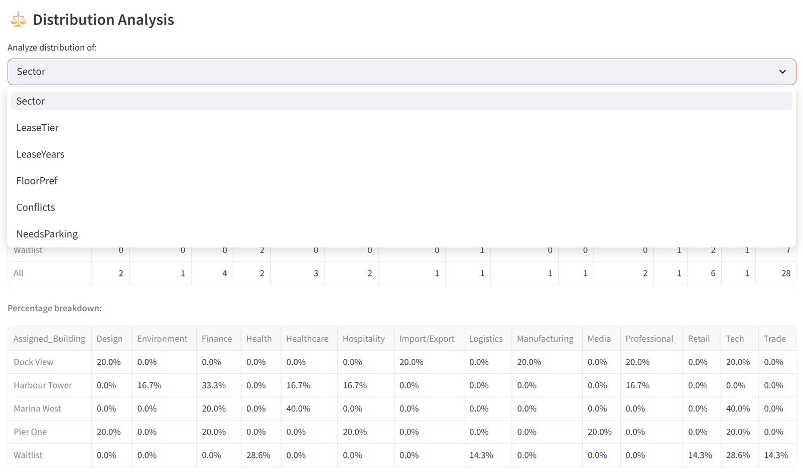
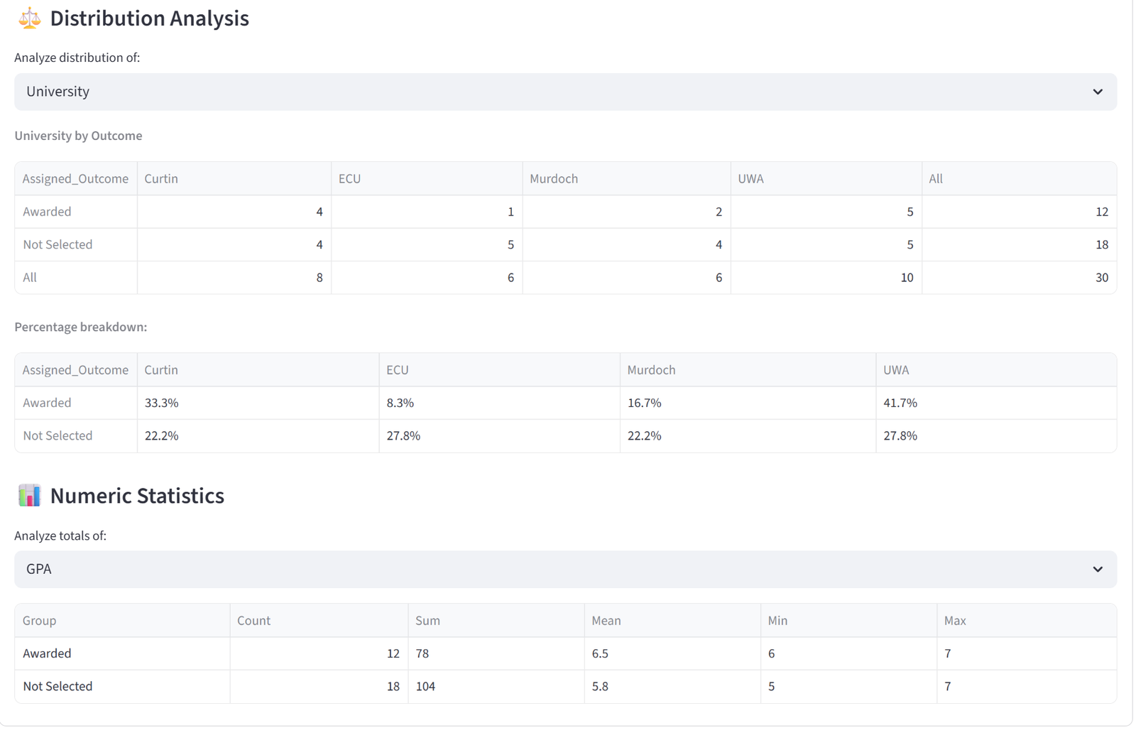
Distribution Analysis provides a dropdown to select any categorical column. Selecting a column generates two tables: a cross-tabulation showing the raw count of each value in each group (with row and column totals), and a percentage breakdown showing the proportion of each value within each group. For example, selecting “Department” shows that Team Alpha is 25% Engineering, 25% Sales, 25% Finance, 25% Operations — or reveals if one department is over-represented.
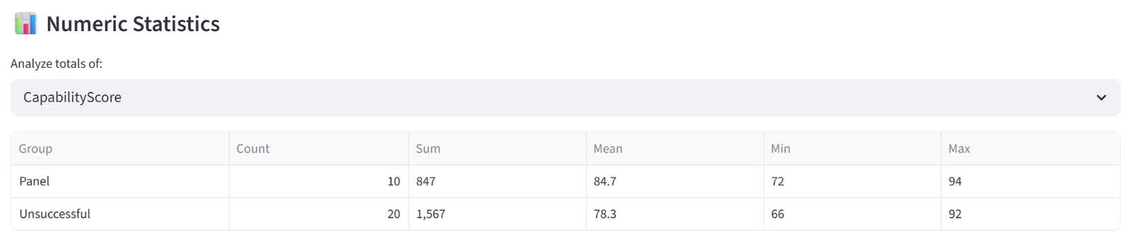
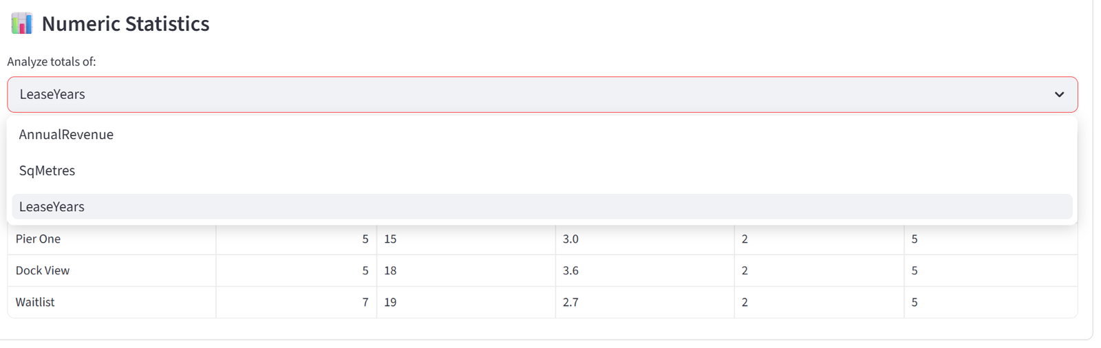
Numeric Statistics provides a similar dropdown for numeric columns. Selecting a column shows a table with each group’s count, sum, mean, min, and max for that column. This is useful for spotting numeric imbalances that aren’t covered by a formal budget constraint — for example, checking average age or experience years across groups even if you didn’t set an explicit rule for it.

These tables are useful for presentations and stakeholder reports. Like all tables in the results, each can be individually exported by hovering and clicking the download icon.

Export

The Export tab provides four download formats, all pre-generated and ready to download instantly.

Excel Report (.xlsx) — a fully formatted workbook containing: a branded Summary sheet with key metrics, a Group Summary sheet showing sizes and budget totals, a Constraints sheet listing every rule you set (budget limits, quotas, preferences, pins, balance rules, relationships) as a complete audit trail, an All Assignments sheet with every item and its assigned group, one sheet per group with just that group’s roster, and distribution cross-tabulation sheets for every categorical column in your data. Headers are styled with branded colours and alternating row shading. This is the most comprehensive export and the one to use for formal reporting or archival.
PDF Rosters — a print-ready branded report with one page per group showing the roster table and summary statistics. Designed to be printed and handed out directly — to teachers, team managers, shift supervisors, or event coordinators.
CSV (All Assignments) — a single flat file with every item and its assigned group column. Opens in any spreadsheet application. Use this for importing into other systems or further processing.
CSV per Group (Zip) — a zip archive containing one CSV file per group, named after the group. Use this when you need to distribute individual rosters to different people — email each team leader their own file.

Tip: Every individual table across all results tabs can also be exported by hovering over it and clicking the download icon — so you can grab a single validation table or a specific analytics cross-tab without downloading the full report.

Sidebar Features

Save & Load

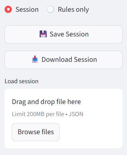
The sidebar has a toggle between Session and Rules only:

Session saves everything: your data and all rules. Use this to pause and resume work.
Rules only saves just the configuration (groups, budgets, quotas, etc.) without data. Use this to apply the same rules to different datasets — for example, running the same classroom placement rules each year with new students.

The Rules Only save is particularly powerful for recurring allocations. A school that runs classroom placement every year can save the rules once (gender balance quotas, IEP budget limits, sibling relationship rules, reading level balance) and reload them the following year with a completely new student list. The rules reference column names, not specific data values, so they apply to any dataset with the same column structure.

The Session save captures a complete snapshot: data, rules, and results. Use this for version control — save before each solver run so you can compare iterations. Name your files descriptively (e.g. “Year6_v1_beforeBalance.json”, “Year6_v2_withPins.json”) for a complete audit trail.

Workflow for applying saved rules to new data: Upload your new data file and import it. Switch the sidebar toggle to “Rules only.” Upload a previously saved rules file. The tool loads the group configuration, budgets, quotas, balance settings, relationships, preferences, and pins — but keeps your new data. Review the rules in each tab to confirm they still make sense with the new data (e.g. column names match), then run the solver.

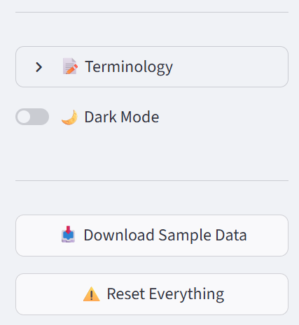
Terminology

Expand the Terminology section to rename the core labels. Change ‘Item’ to ‘Student’, ‘Group’ to ‘Class’, and ‘ID’ to ‘Student ID’. This updates labels throughout the interface.

Dark Mode

Toggle for a dark colour scheme. Purely cosmetic.

Sample Data & Reset

Download Sample Data provides a small CSV to test with. Reset Everything clears all data and settings — use with caution.

Tips & Best Practices

Start simple, add complexity. Begin with just groups and capacity. Run the solver. Then add one constraint type at a time. This lets you identify which rule causes issues if the solver reports infeasibility.
Use soft constraints when possible. Hard constraints (must enforce, pins) reduce the solver’s options. Soft constraints (preferences, flexible capacity) give better results because the solver has more room to optimise.
Check the Validation tab. After every run, review which constraints passed and which were partially met. This tells you exactly where compromises were made.
Save before you run. Use the session save so you can revert if the results are not what you expected.
Increase the timeout for large problems. 700+ items with many constraints may need 60–90 seconds. Check the Options tab.
Name your groups meaningfully. ‘Mrs Robertson’ is more useful than ‘Group 1’ when reviewing results.
Use the priority sliders wisely. If relationships are more important than balance, increase Keep Apart/Together and decrease Balance.
Understand the difference between hard and soft. Budgets, required relationships, and pins are hard — the solver fails if it can’t satisfy them. Balance, preferences, and soft relationships are soft — the solver does its best but can compromise. If you’re getting infeasible results, check whether you’ve made too many things hard.
Use Tags for group categories. Instead of applying a quota to each group individually, tag groups (e.g. “Division 1”, “Active”, “Ground Floor”) and apply rules to the tag. This scales better and is easier to maintain when you add or rename groups.
The select/reject pattern works for any competitive selection. Create two groups: one for selected items (fixed size) and one for the remainder. Use Maximise on a merit column targeting the selected group. Add quotas for diversity requirements. This works for scholarships, grants, team selection, shortlisting, and any scenario where you’re picking the best N from a pool.
Combined budgets are for shared resources. If two buildings share a parking structure, or two shifts share an equipment pool, use a combined budget rather than trying to calculate individual limits. The solver handles the allocation within the shared cap.
Don’t over-constrain. Every hard constraint reduces the solver’s options. If you set hard quotas, hard budgets, hard relationships, and pins all at once on a small dataset, the solver may report infeasibility simply because there aren’t enough items to satisfy every rule simultaneously. Start with the most important constraints as hard, and make everything else soft.
Check the constraint summary line. Before clicking Run, scan the summary below the Configuration section. If it shows 0 quotas when you expected 3, you probably forgot to click the Add button after filling in the quota form.

Troubleshooting

Problem	Cause	Fix
No Solution Possible	Hard constraints conflict	Review conflict report. Relax hard quotas, reduce pins, or increase capacity.
‘Good’ instead of ‘Optimal’	Solver ran out of time	Increase timeout in Options tab. Or accept the ‘Good’ solution — it is valid.
Relationships not working	IDs in the relationship column don’t match the ID column	Ensure IDs match exactly (case-sensitive). Check the separator character.
Balance seems uneven	Balance weight is too low	Increase the Balance priority slider in Options. Or the data itself may be skewed.
Data upload errors	Wrong file format or encoding	Save as CSV UTF-8 from Excel. Remove merged cells or empty header rows.
Solver takes too long	Too many items or constraints	Increase timeout in Options. Reduce hard constraints. For 500+ items, start with 60–90 seconds.
Pins conflict with relationships	A pinned item’s partner can’t fit in the same group	Reduce pins. Use preferences instead where possible. Check that pinning doesn’t force more items into a group than its capacity allows.
Quotas don’t seem to apply	Quota targets the wrong groups or mode	Check the Apply to dropdown. Check Percentage vs Count mode. Verify you clicked Add after filling in the form.
Budget values reset after changing group count	Editor state not committed before resize	This is fixed in the latest version. If you experience it, save your session before changing group count.
Relationship warning about unknown IDs	Column has labels instead of IDs	The relationship column must contain item IDs (e.g. G004), not shared labels (e.g. Taylor). See the Relationships section.

Getting Help

If you encounter a bug, unexpected behaviour, or need assistance with your allocation, visit the website balancedapp.io for additional information or contact us at support@balancedapp.io.

When reporting an issue, include the following so we can help quickly:

A description of what you were trying to do and what happened instead
The error message, if one appeared (a screenshot is ideal)
Your saved session file (.json) — use the Session save in the sidebar to capture your data and rules at the point the issue occurred
The number of items and groups you were working with
Your browser (Chrome, Safari, Edge, etc.)

We also welcome feature requests and feedback on the tool. If you have a use case that doesn’t quite fit the current feature set, let us know — many of the features in this version were built in response to user feedback.

Glossary

Term	Definition
Item	A single thing being allocated (a student, a package, a nurse)
Group	A container items are assigned to (a class, a truck, a shift)
Budget	A numeric column limit per group (e.g. max weight, salary cap)
Combined Budget	A shared budget across multiple groups
Quota	A percentage or count requirement per group (e.g. 40–60% female)
Balance	Evening out the distribution of a column across groups
Relationship	A keep-apart or keep-together rule based on item ID references
Preference	A soft or hard rule that items matching a condition should go to a specific group
Pin	A hard assignment of a specific item to a specific group
Exclusion	A hard rule preventing an item from being in a specific group
Tag	A label on a group used to target rules at multiple groups
Flex	Soft capacity on a group — the solver can slightly exceed the limit
Hard constraint	Must be satisfied — solver fails if it cannot
Soft constraint	Preferred but can be violated if necessary
Feasible	A valid solution that satisfies all hard constraints
Optimal	The mathematically best feasible solution

Worked Examples

The following eight appendices provide complete, realistic scenarios with sample data and step-by-step instructions. Additional examples and a copy of each CSV file is available for download from balancedapp.io.

Appendix A: Education — Classroom Placement

Scenario

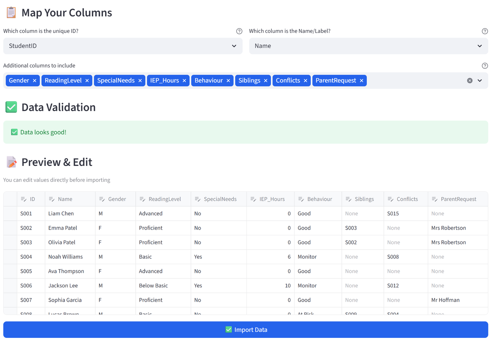
Greenfield Primary School needs to form 4 classes of 8 students from 32 incoming Year 3 students. Classes must be balanced by gender and reading level. Students with special needs require IEP (Individual Education Plan) hours, and no class should bear a disproportionate load. Certain students have documented behavioural conflicts. Siblings must be kept together. Some parents have requested specific teachers.

The data includes 32 students with gender, reading level (Advanced/Proficient/Basic/Below Basic), special needs status, IEP hours, behaviour flags, sibling links, conflict links, and parent teacher requests.

The Data

Save the following as classroom_placement.csv:

32 rows, 10 columns. First 5 rows shown:

StudentID	Name	Gender	ReadingLevel	SpecialNeeds	IEP_Hours	Behaviour	Siblings	Conflicts	ParentRequest
S001	Liam Chen	M	Advanced	No	0	Good		S015
S002	Emma Patel	F	Proficient	No	0	Good	S003		Mrs Robertson
S003	Olivia Patel	F	Proficient	No	0	Good	S002		Mrs Robertson
S004	Noah Williams	M	Basic	Yes	6	Monitor		S008
S005	Ava Thompson	F	Advanced	No	0	Good

Full CSV file: classroom_placement.csv

Step-by-Step Instructions

Step 1: Upload & Map

Upload classroom_placement.csv.
Set Unique ID to StudentID and Display Name to Name.
Keep all columns. Click Import Data.

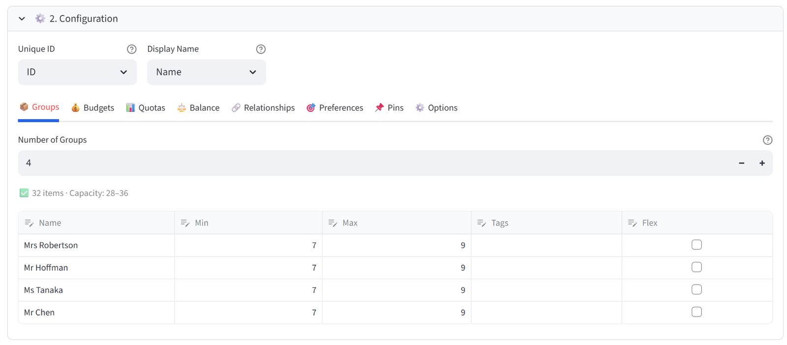
Step 2: Configure Groups

Set Number of Groups to 4.
Rename to: Mrs Robertson, Mr Hoffman, Ms Tanaka, Mr Chen.
Set each to Min 7 / Max 9.

Step 3: Set Budget — IEP Hours

Go to the Budgets tab.
Select IEP_Hours from the multiselect.
Set Max Total to 25 for each class (prevents overloading any one teacher).
Leave Min Total at 0.

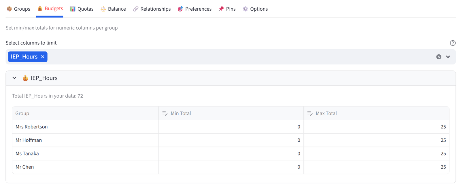
Tip: Total IEP hours across all students is 72. With a max of 25 per class, the solver must spread them across at least 3 classes.

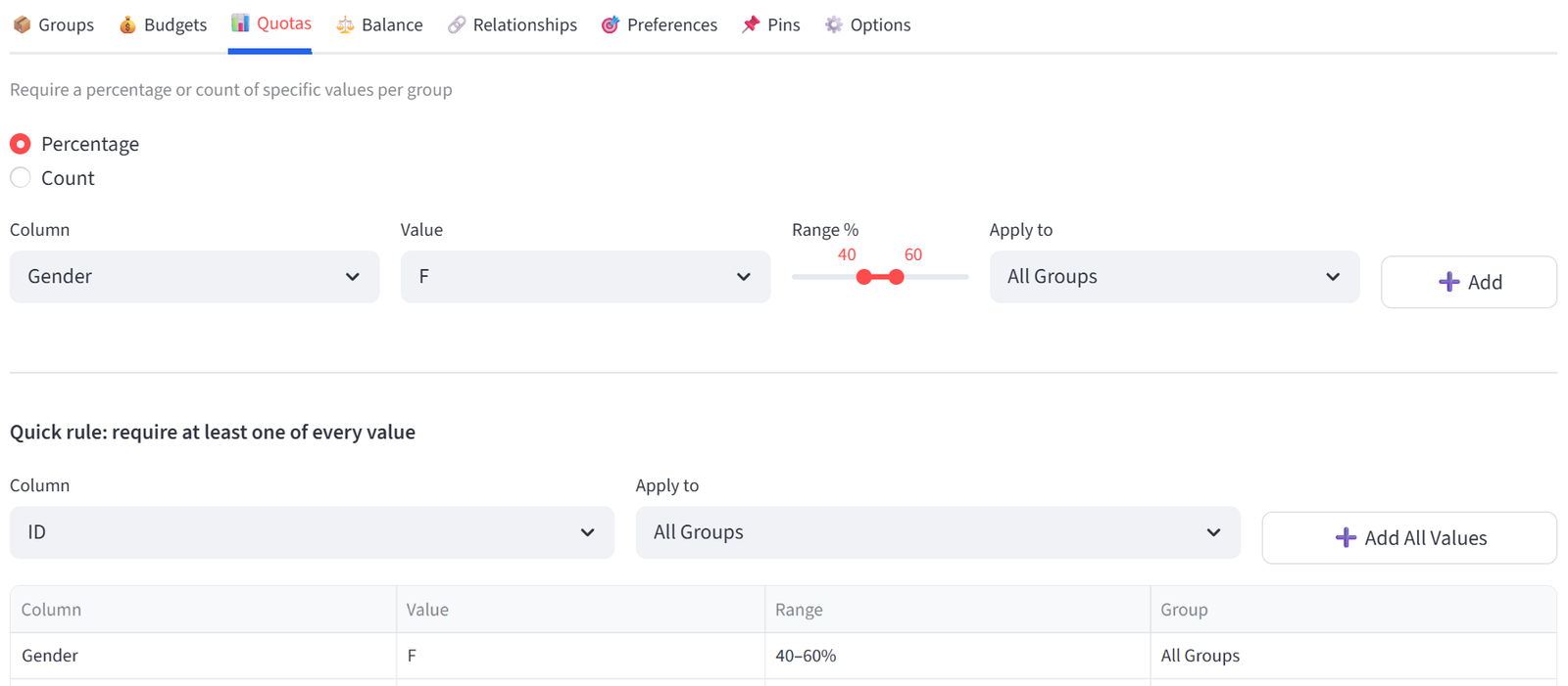
Step 4: Set Quotas — Gender Balance

Go to the Quotas tab. Ensure Percentage mode is selected.
Column: Gender, Value: F, Min: 40, Max: 60. Group: All Groups. Click Add.
This ensures every class is 40–60% female. The balance male, which will inherently be 40–60% given there are two options which will total to 100%. This means we do not technically need to set a second 40-60% male rule, though it can be inserted if desired.

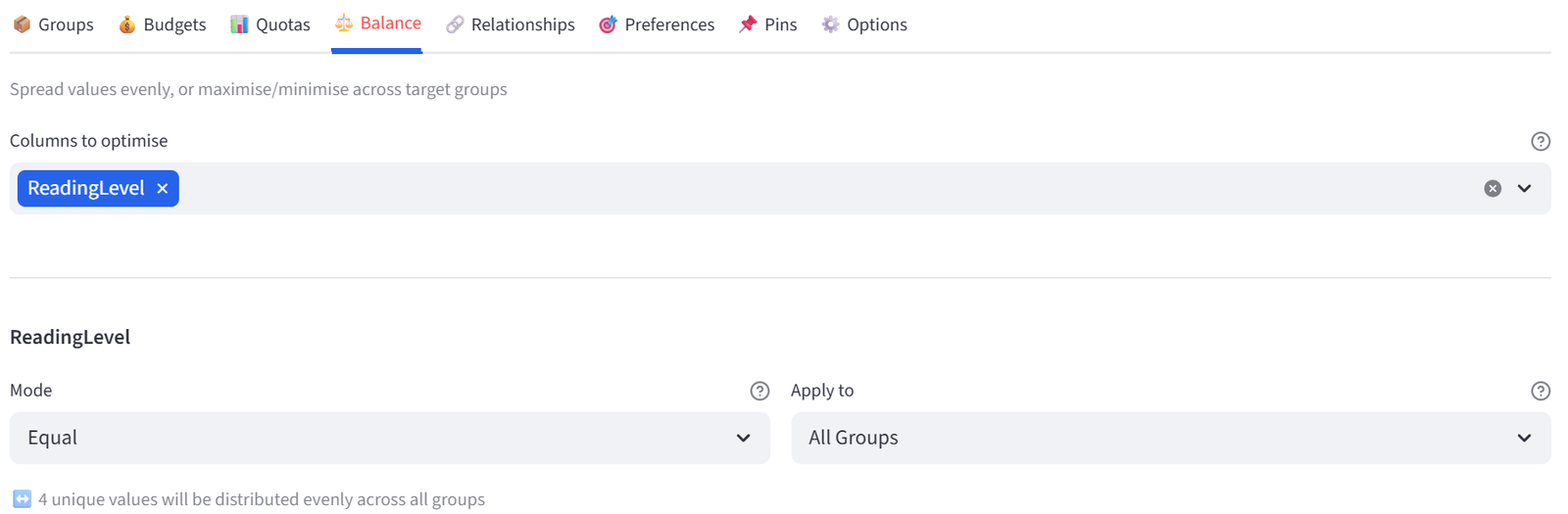
Step 5: Enable Balance — Reading Level

Go to the Balance tab.
Select ReadingLevel from the multiselect.
Leave mode as Equal and apply to All Groups. This spreads Advanced, Proficient, Basic, and Below Basic students evenly across all 4 classes.

Step 6: Add Relationships — Conflicts and Siblings

Go to the Relationships tab.
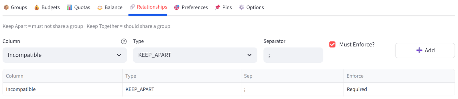
Add rule: Column = Conflicts, Type = KEEP_APART, Enforce = Required. Click Add.
Add rule: Column = Siblings, Type = KEEP_TOGETHER, Enforce = Required. Click Add.

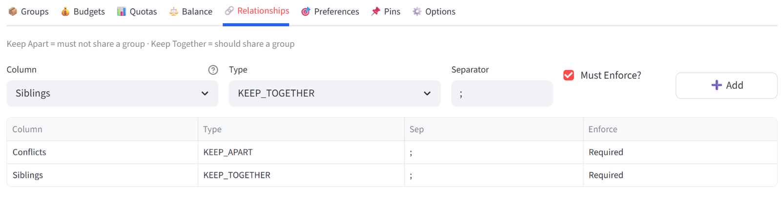
Tip: S002 and S003 (the Patel sisters) will be kept together. S001 and S015 (a documented conflict) will be separated.

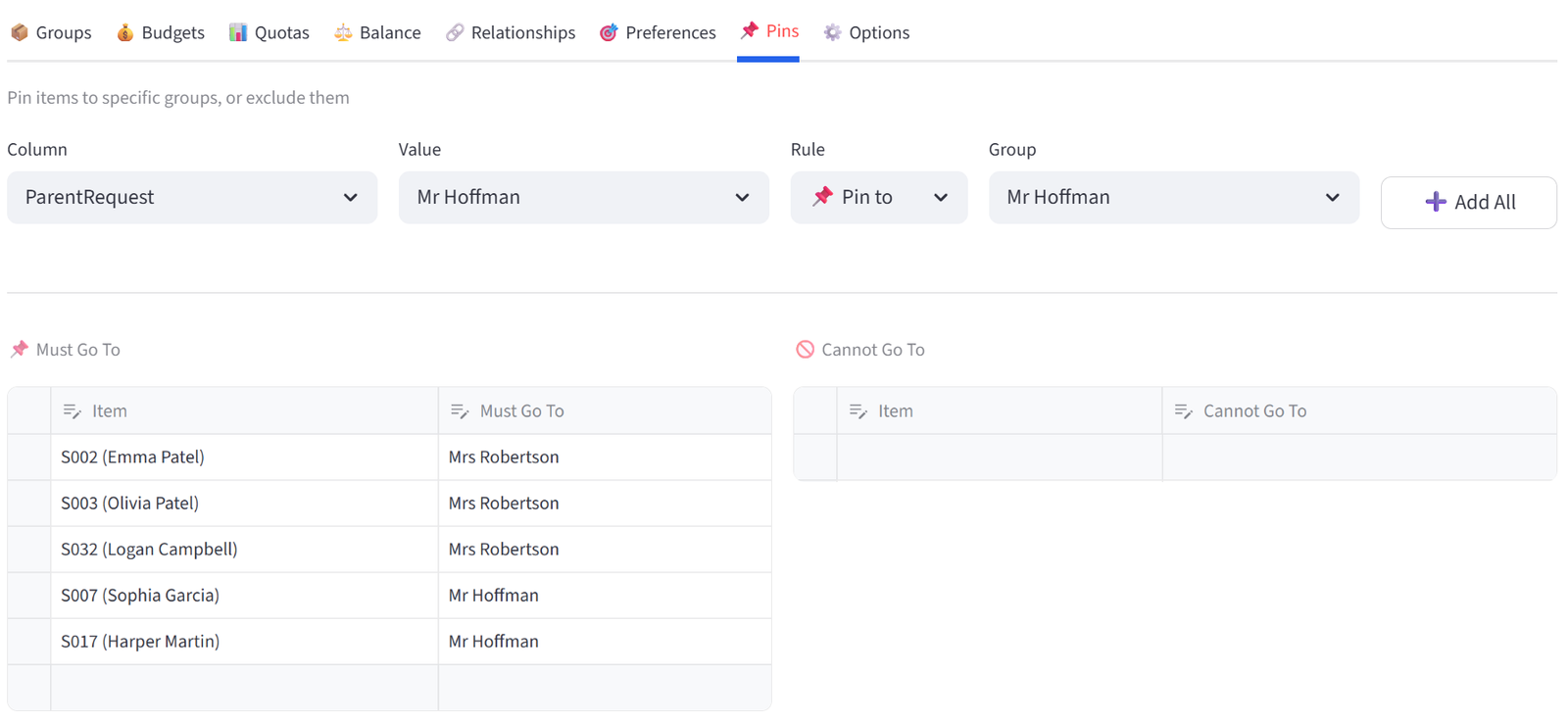
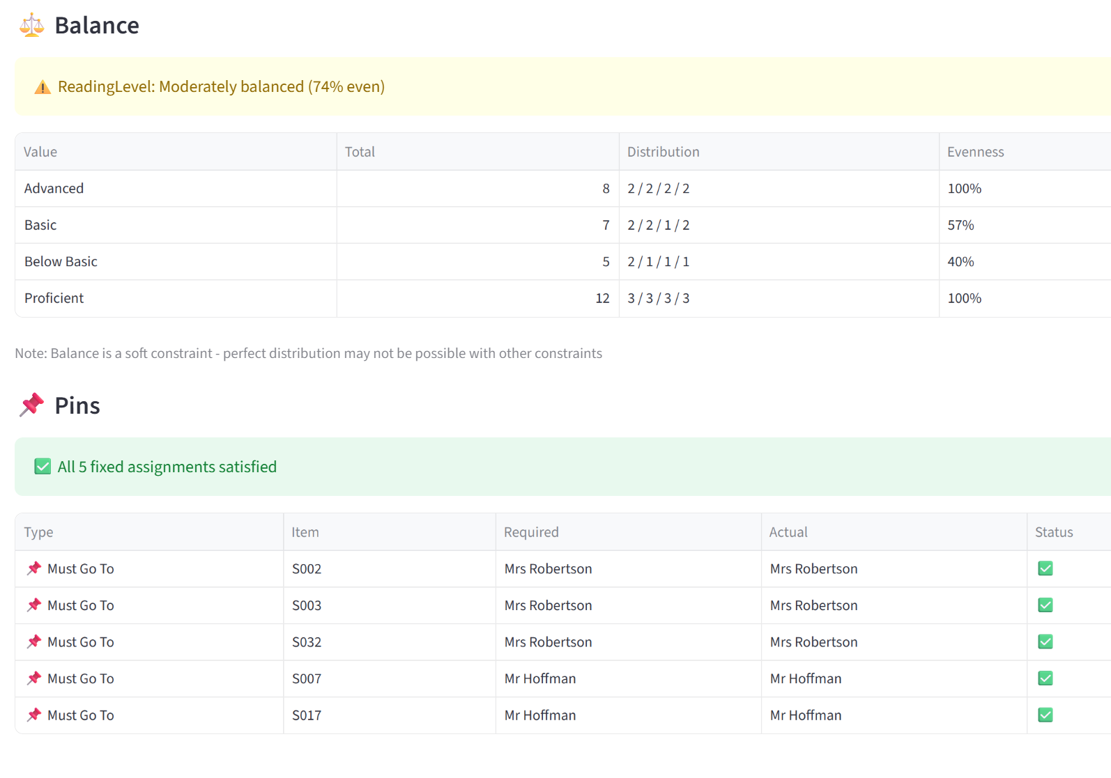
Step 7: Add Pins — Parent Requests

Go to the Pins tab.
Use Bulk Assign: Column = ParentRequest, Value = Mrs Robertson, Rule = Pin to, Group = Mrs Robertson. Click Add All.
Repeat for Mr Hoffman.
This pins S002, S003, S032 to Mrs Robertson and S007, S017 to Mr Hoffman.

Step 8: Run the Optimiser

Scroll to the Run Optimizer button and click it.
The solver should find an Optimal or Good solution within a few seconds.

Step 9: Validate & Export

Check the Validation tab: all quotas, budgets, and relationships should pass.
Review the Analytics tab to see gender and reading level distribution charts.
Export as Excel and share with the teaching team.

Expected Outcome

Each class has 7–9 students. Gender is 40–60% female in every class. Reading levels are spread evenly. No class exceeds 25 IEP hours. Siblings (Patels, Browns, Scotts, Harrises) are together. Conflict pairs are separated. Parent-requested students are in the right class.

If the solver reports Good rather than Optimal, the result is still valid — it means the time limit was reached before proving mathematical optimality, but all hard constraints are satisfied.

This example uses 32 students for clarity, but schools routinely run this with 100–700+ students across 4–28 classes using the same rule setup. Increase the solver timeout in Options for larger cohorts. Use the Rules Only save to preserve this year’s configuration and reload it next year with a fresh student list.

Appendix B: Events — Wedding Seating

Scenario

James and Sophie are getting married with 30 guests seated at 3 tables of 10. Requirements: bridal party at Table 1 (the top table), families together, exes apart, a mix of both sides at each table, and dietary needs spread so the kitchen can manage service. VIPs should be close to the couple.

The data includes 30 guests with side (Bride/Groom), table group (Friends/Family/Work), dietary requirements, age, family groupings, ex-partner conflicts, bridal party role, and VIP status.

The Data

Save the following as wedding_seating.csv:

30 rows, 10 columns. First 5 rows shown:

GuestID	Name	Side	TableGroup	Dietary	Age	Family	Exes	BridalParty	VIP
G001	James Mitchell	Groom	Friends	None	32			Best Man	Yes
G002	Sarah Mitchell	Groom	Friends	Vegetarian	30
G003	Robert Taylor	Bride	Family	None	58	Taylor		Father of Bride	Yes
G004	Linda Taylor	Bride	Family	Gluten Free	56	Taylor		Mother of Bride	Yes
G005	Michael Chen	Groom	Family	None	61	Chen			Yes

Full CSV file: wedding_seating.csv

Step-by-Step Instructions

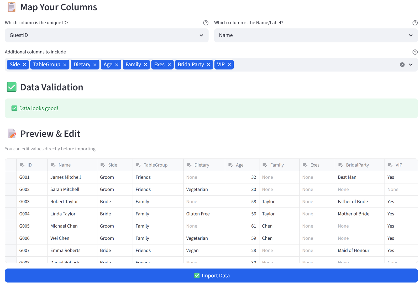
Step 1: Upload & Map

Upload wedding_seating.csv.
Set Unique ID to GuestID and Display Name to Name.
Keep all columns. Click Import Data.

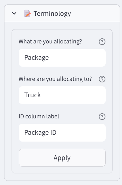
Step 2: Set Terminology

In the sidebar, expand Terminology.
Change Item to ‘Guest’, Group to ‘Table’, ID to ‘Guest ID’. Click Apply.

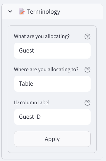
Tip: The entire interface now reads ‘Guest’ and ‘Table’ instead of ‘Item’ and ‘Group’.

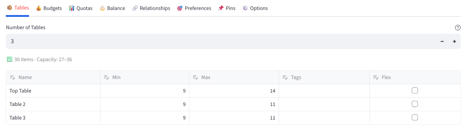
Step 3: Configure Tables

Set Number of Tables to 3.
Rename to: Top Table, Table 2, Table 3.
Set the Top Table to Min 9 / Max 14 and each to Min 9 / Max 11.

Step 4: Pin Bridal Party

Go to the Pins tab.
Bulk Assign: Column = BridalParty, Value = Best Man, Rule = Pin to, Group = Top Table. Click Add All.
Repeat for Maid of Honour, Father of Bride, Mother of Bride.

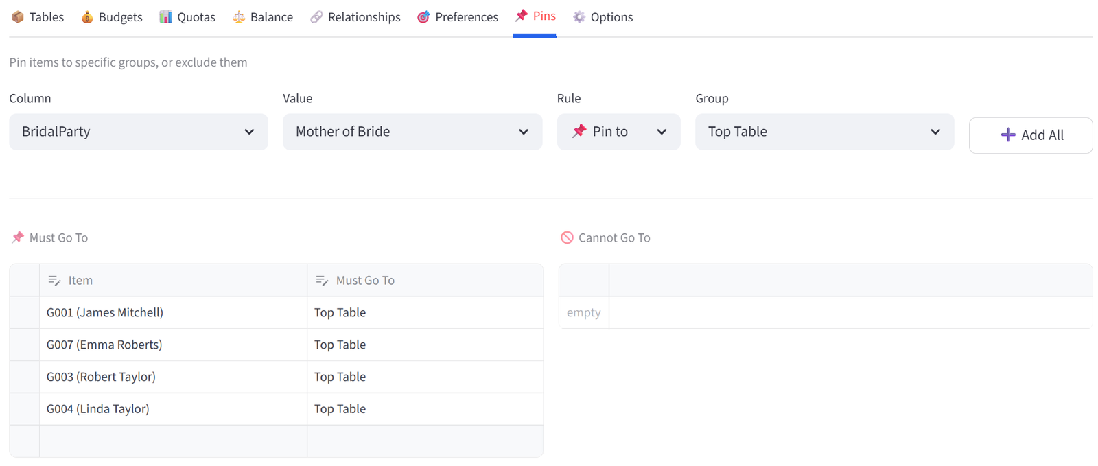
Tip: This gives the Top Table its bridal party core. We have excluded the groomsman and bridesmaids to allow them to be paired with their partners across any of the three tables. The solver fills remaining seats optimally.

Step 5: Add Relationships

Go to the Relationships tab.
Add: Column = Family, Type = KEEP_TOGETHER, Enforce = Required.
Add: Column = Exes, Type = KEEP_APART, Enforce = Required.

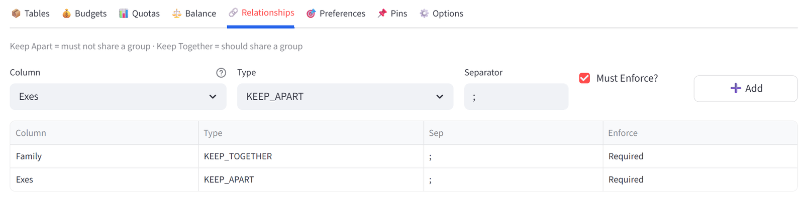
Tip: The Family column contains the Guest IDs of family members (e.g. G003 has G004, meaning Robert and Linda Taylor must sit together). This is how relationships work — the column must contain IDs of other items, not shared labels. The Exes column works the same way: G013 lists G025, keeping Tom Davies and Ryan Hughes apart.

Step 6: Set Balance — Side Mix

Go to the Balance tab.
Select Side. Leave mode as Equal.
This ensures each table has a mix of Bride-side and Groom-side guests.

Step 7: Set Quota — Dietary Spread

Go to the Quotas tab. Select Count mode.
Column: Dietary, Value: Vegan, Min: 0, Max: 2. Group: All Tables. Click Add.
Column: Dietary, Value: Vegetarian, Min: 0, Max: 3. Group: All Tables. Click Add.

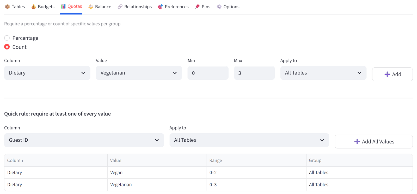
Tip: This prevents all special diets from landing at one table, helping kitchen logistics.

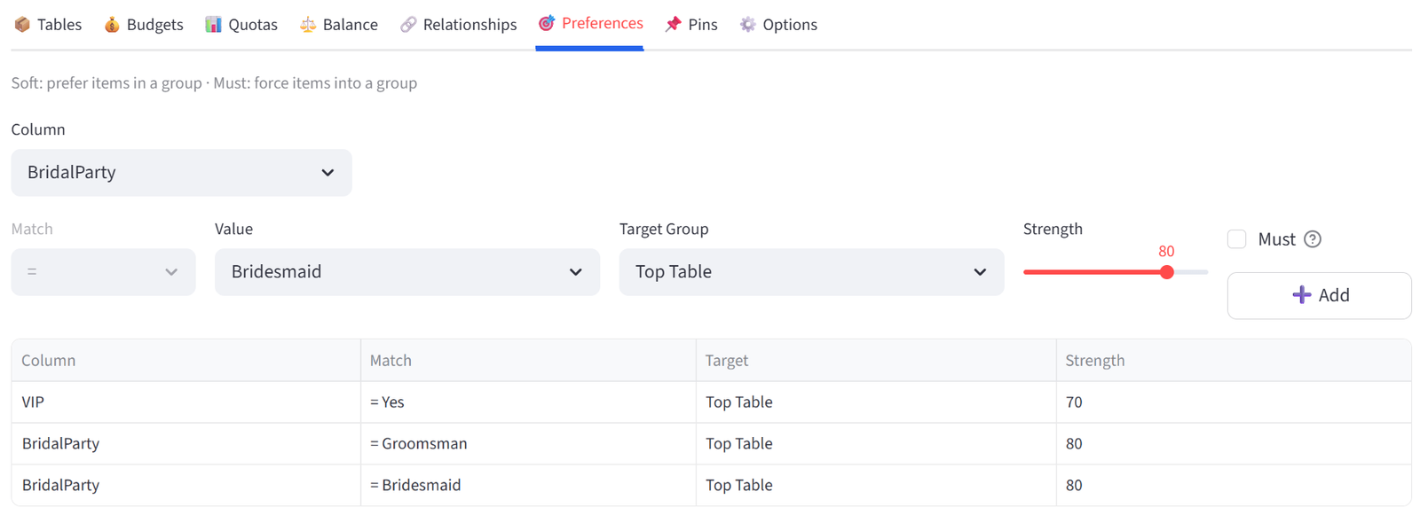
Step 8: Add Preference — VIPs

Go to the Preferences tab.
Column: VIP, Operator: =, Value: Yes, Target: Top Table, Strength: 70. Click Add.
This gives a strong but not mandatory pull for VIPs to the top table.
Column: BridalParty, Operator: =, Value: Groomsman, Target: Top Table, Strength: 80. Click Add.
Column: BridalParty, Operator: =, Value: Bridesmaid, Target: Top Table, Strength: 80. Click Add.
This gives a very strong but not mandatory pull for the remaining bridal party to the top table.

Step 9: Run & Validate

Click Run Optimizer.
Check Validation: families together, exes apart, dietary quotas met, sides balanced.
Export as PDF for the venue coordinator.

Expected Outcome

The Top Table seats the majority of bridal party, parents, and some VIPs. Each table has a mix of Bride and Groom guests. Where groomsman or bridesmaids are not on the Top Table, they are with their family. Family members are together. Tom Davies (G013) and Ryan Hughes (G025) are at separate tables. No table has more than 2 vegans or 3 vegetarians.

The solver balances these competing requirements simultaneously — something that would take hours by hand with 30 guests and is practically impossible with 150+. This example uses 30 guests at 3 tables, but the same rules work for 150 guests at 15 tables or 300 guests at 30 tables. Only the data file and number of groups change.

Appendix C: Logistics — Fleet Loading

Scenario

Metro Distribution has 24 packages to load onto 4 trucks. Each truck has a weight limit and volume limit. Packages have destination zones (CBD, North, South, East, West), priority levels, fragile flags, and hazardous material classifications. The goal is efficient loading that respects all limits while spreading fragile items to reduce risk.

The data includes 24 packages with weight (kg), volume (m³), destination zone, priority, fragile flag, hazard class, and special handling notes.

The Data

Save the following as fleet_loading.csv:

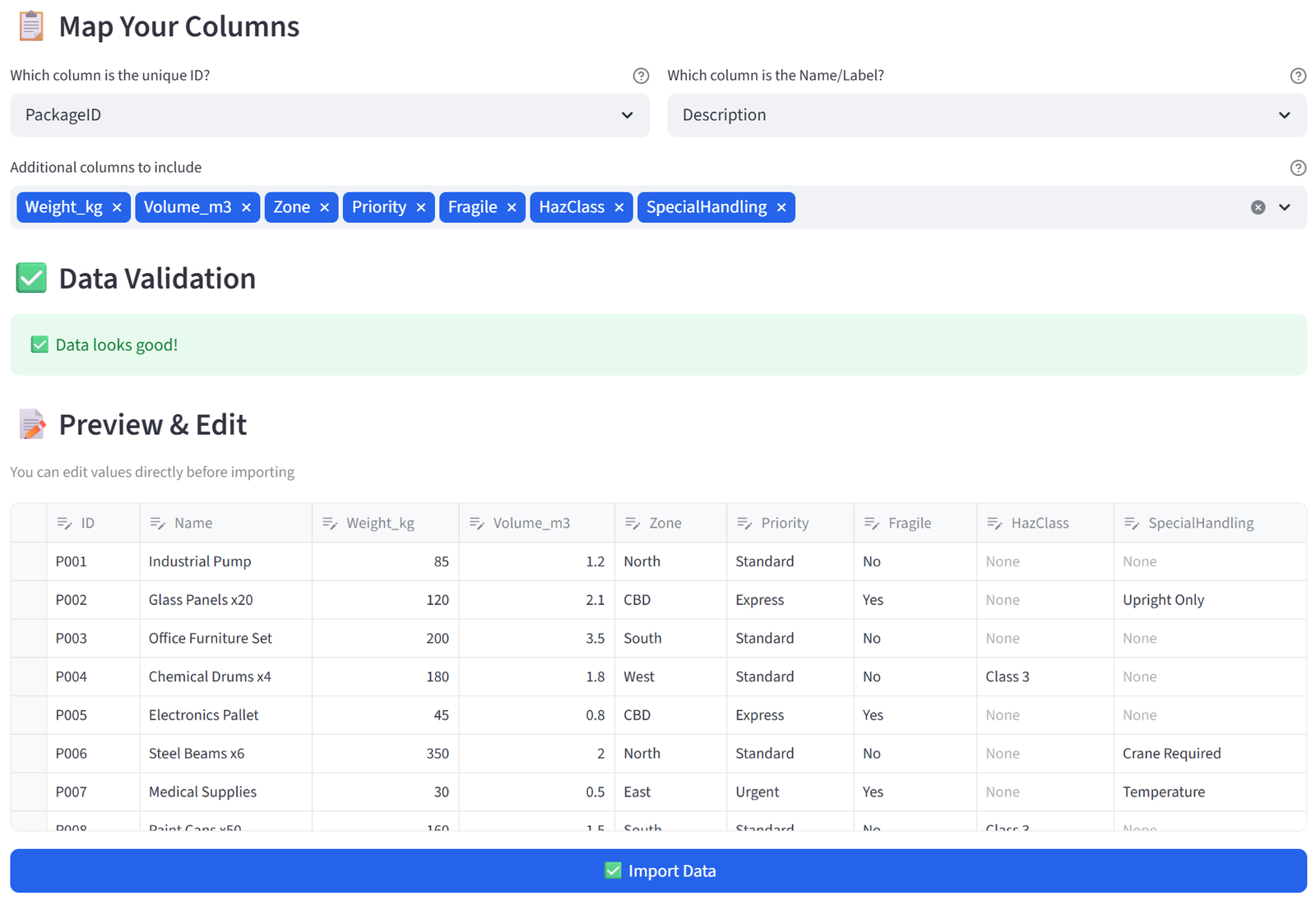
24 rows, 9 columns. First 5 rows shown:

PackageID	Description	Weight_kg	Volume_m3	Zone	Priority	Fragile	HazClass
P001	Industrial Pump	85	1.2	North	Standard	No	None
P002	Glass Panels x20	120	2.1	CBD	Express	Yes	None
P003	Office Furniture Set	200	3.5	South	Standard	No	None
P004	Chemical Drums x4	180	1.8	West	Standard	No	Class 3
P005	Electronics Pallet	45	0.8	CBD	Express	Yes	None

Full CSV file: fleet_loading.csv

Step-by-Step Instructions

Step 1: Upload & Map

Upload fleet_loading.csv.
Set Unique ID to PackageID, Display Name to Description.
Keep all columns. Click Import Data.

Step 2: Set Terminology

Change Item to ‘Package’, Group to ‘Truck’, ID to ‘Package ID’.

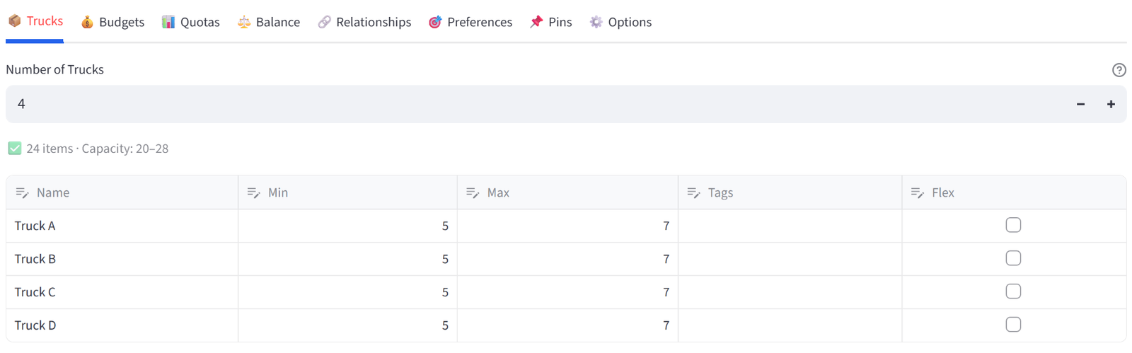
Step 3: Configure Trucks

Set Number of Trucks to 4.
Rename to: Truck A, Truck B, Truck C, Truck D.
Set each to Min 5 / Max 7.

Step 4: Set Budgets — Weight and Volume

Go to the Budgets tab.
Select Weight_kg. Set Max Total to 1500 for each truck.
Select Volume_m3. Set Max Total to 12.0 for each truck.

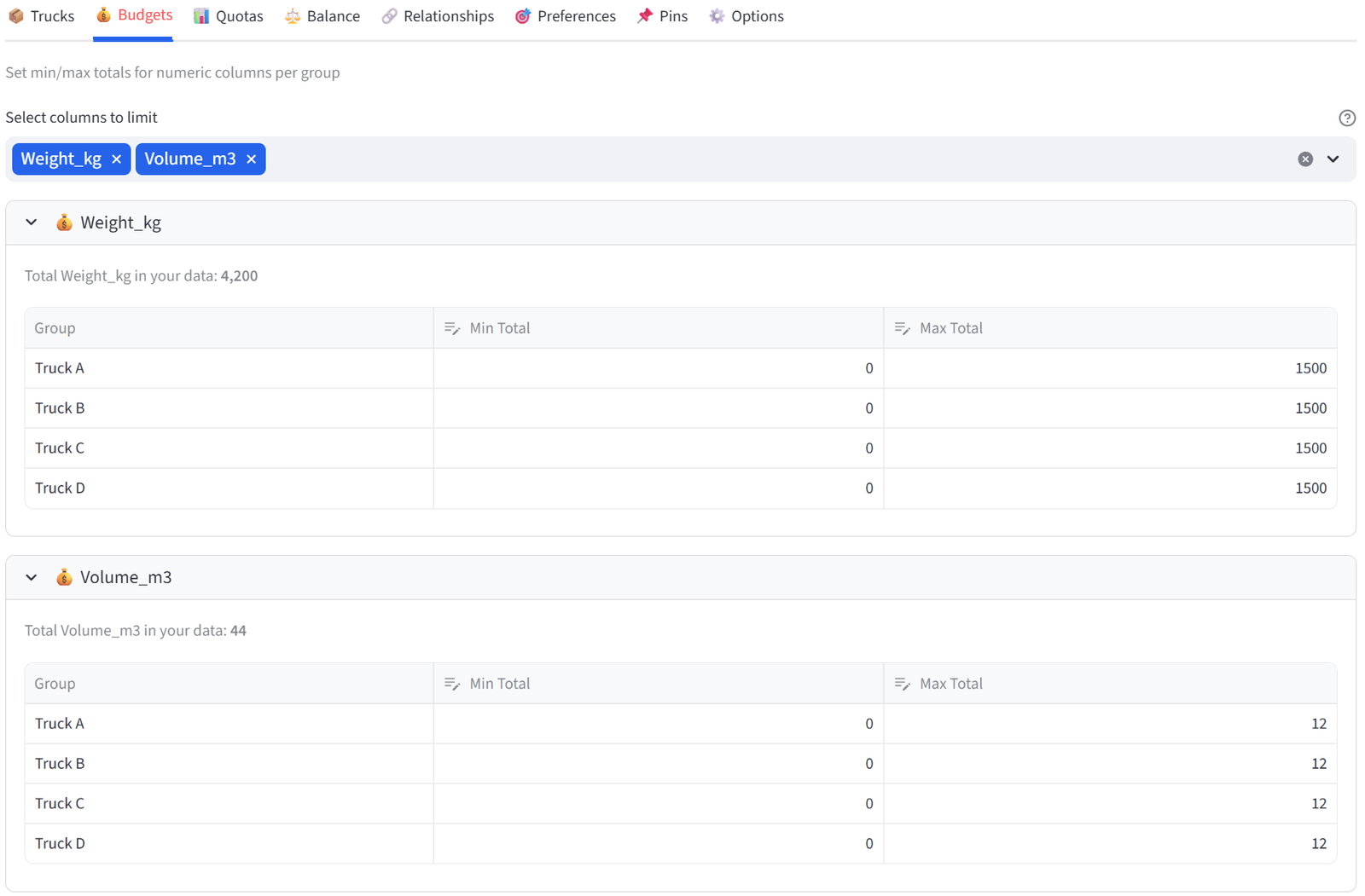
Tip: Total weight is ~4,200kg across 24 packages. With 4 trucks at max 1,500kg each, there is enough capacity but the solver must balance carefully.

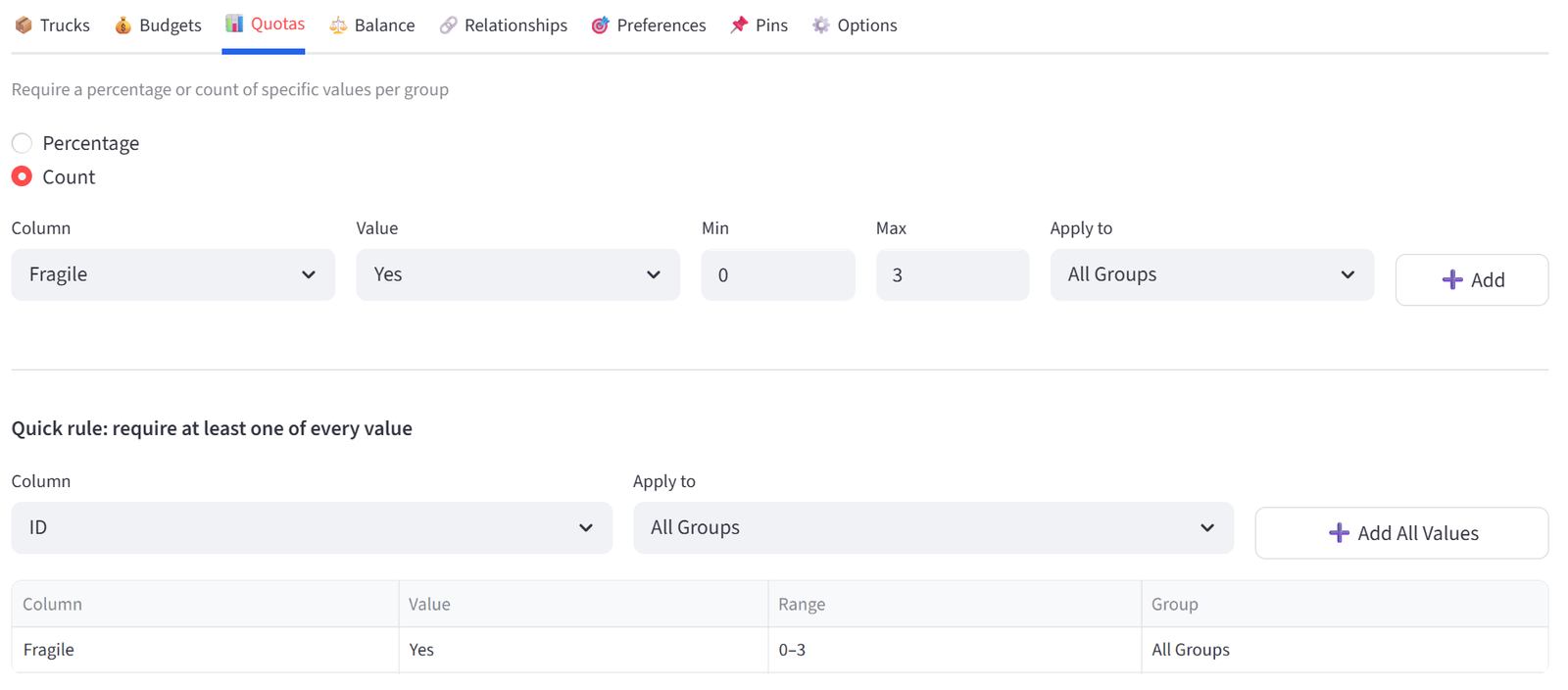
Step 5: Set Quota — Fragile Spread

Go to the Quotas tab. Use Count mode.
Column: Fragile, Value: Yes, Min: 0, Max: 3. Group: All Trucks. Click Add.

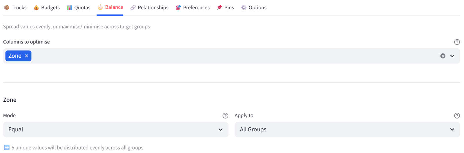
Step 6: Set Balance — Zones

Go to the Balance tab.
Select Zone. Leave mode as Equal.
This spreads destination zones across trucks, which helps with delivery routing.

Step 7: Add Preference — CBD Express on Truck A

Go to the Preferences tab.
Column: Zone, Operator: =, Value: CBD, Target: Truck A, Strength: 80. Click Add.
Column: Priority, Operator: =, Value: Urgent, Target: Truck A, Strength: 90. Click Add.

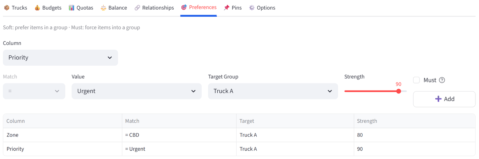
Tip: Truck A departs first and covers CBD. Urgent items get priority loading.

Step 8: Minimise Hazmat on Truck D

Go to the Balance tab.
Select HazScore from the multiselect.
Set Mode to Minimise. Set Target group to Truck D.

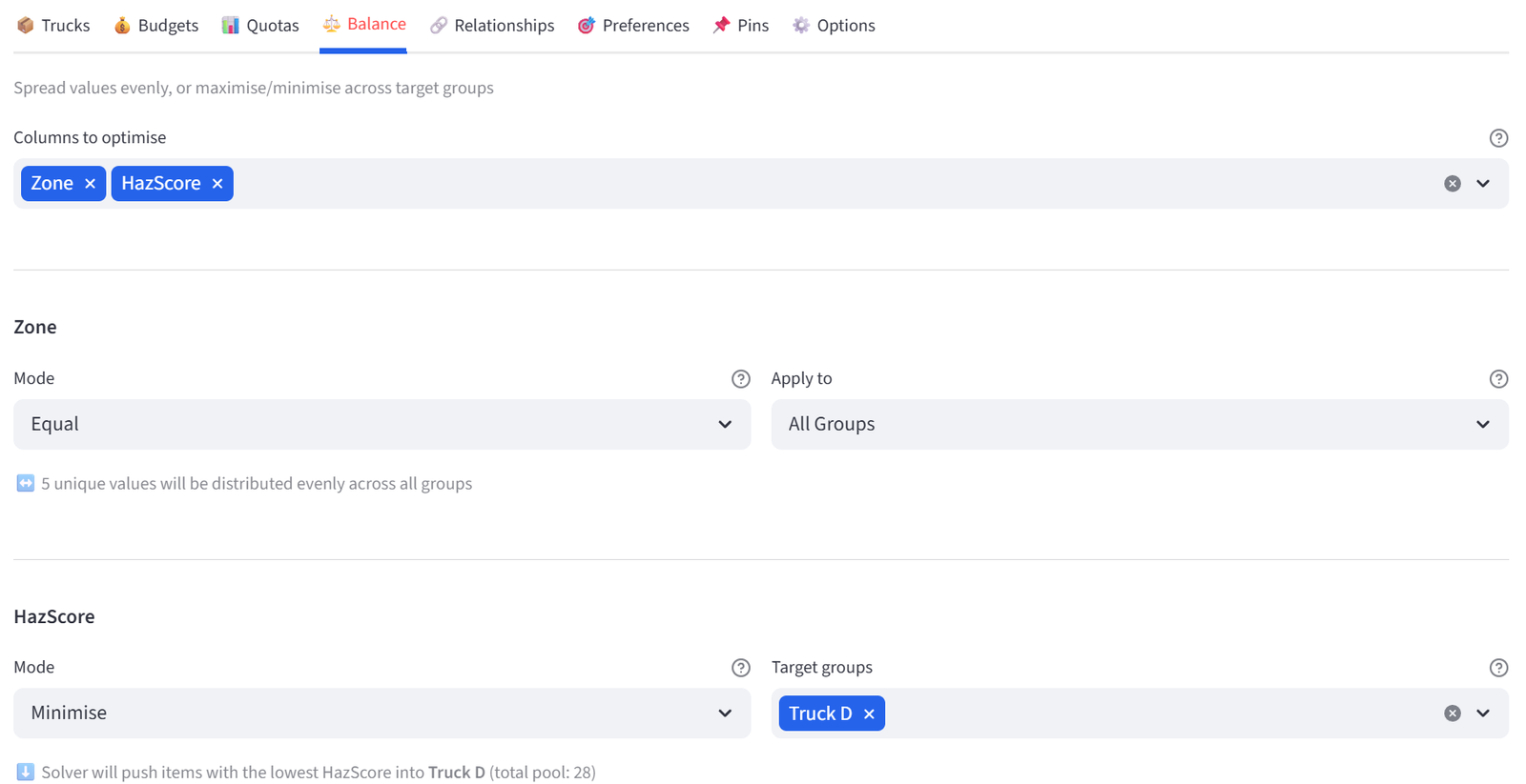
Tip: Truck D is the oldest vehicle with the least hazmat containment. HazScore is a numeric column (0 for non-hazardous, 3/5/8/9 matching the UN hazard class). Minimise works on numeric columns by reducing the total sum in the target group — so it pushes high-scoring hazmat packages away from Truck D toward the other trucks. If your data only has text labels (like HazClass), you need to add a numeric equivalent for Maximise/Minimise to work.

Step 9: Run & Validate

Click Run Optimizer.
Check Validation: no truck exceeds weight/volume limits, fragile items are spread, zone balance is reasonable, Truck D has few or no hazmat packages.
Export for the dispatch team.

Expected Outcome

No truck exceeds 1,500kg or 12.0m³. Fragile items are spread across trucks (max 3 per truck). CBD and Urgent packages cluster toward Truck A. Truck D has minimal or no hazardous materials. Zone distribution is roughly even. Each truck has 5–7 packages.

The solver handles the multi-dimensional packing problem (weight + volume + zone + priority + fragility + hazmat) in seconds. Manual loading would require constant recalculation as each package is assigned.

This example uses 24 packages for clarity, but the same configuration scales to hundreds of packages across dozens of vehicles with no changes to the rule setup — only the data file grows.

Appendix D: Healthcare — Shift Scheduling

Scenario

City General Hospital needs to assign 30 nurses across 3 shifts (Day, Evening, Night). Each shift needs a mix of certifications (RN, LPN), specialties, and seniority levels. Each shift has a patient load hour budget. At least one Charge Nurse per shift is required. Certain nurse pairs have requested not to work together.

The data includes 30 nurses with certification, specialty, seniority, years of experience, patient load hours, incompatible pairs, and charge nurse flags.

The Data

Save the following as shift_scheduling.csv:

30 rows, 9 columns. First 5 rows shown:

NurseID	Name	Certification	Specialty	Seniority	Years	PatientLoadHrs	Incompatible	ChargeNurse
N001	Anna Morrison	RN	Emergency	Senior	18	22		Yes
N002	Ben Cooper	RN	ICU	Senior	15	20	N005	Yes
N003	Clara Dunn	LPN	General	Mid	8	16
N004	Derek Fong	RN	Paediatrics	Senior	20	18		Yes
N005	Elena Ruiz	RN	ICU	Mid	6	18	N002

Full CSV file: shift_scheduling.csv

Step-by-Step Instructions

Step 1: Upload & Map

Upload shift_scheduling.csv.
Set Unique ID to NurseID, Display Name to Name.
Import all columns.

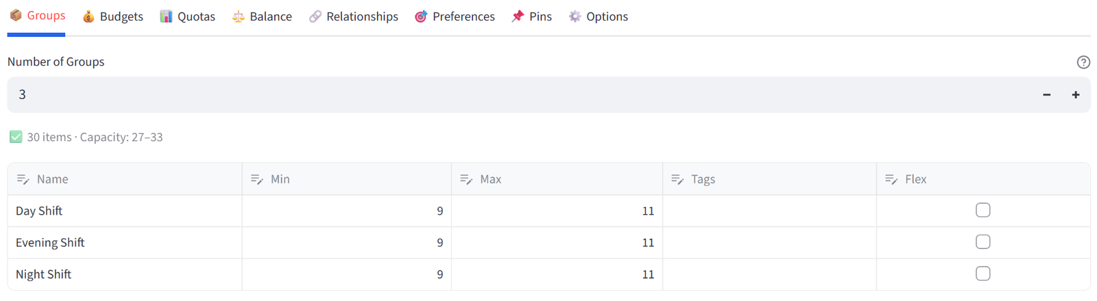
Step 2: Configure Shifts

Set Number of Groups to 3.
Rename to: Day Shift, Evening Shift, Night Shift.
Set each to Min 9 / Max 11.

Step 3: Set Budget — Patient Load Hours

Go to Budgets tab. Select PatientLoadHrs.
Set Min Total to 140, Max Total to 180 for each shift.

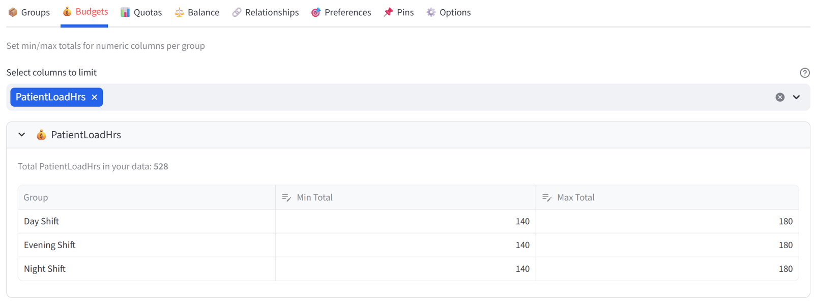
Tip: Total patient load hours across all nurses is ~520. With 3 shifts at 140–180 each, coverage is 420–540.

Step 4: Set Quotas

Go to Quotas tab. Use Count mode.
Column: ChargeNurse, Value: Yes, Min: 2, Max: 4. Group: All Groups. Click Add.
Switch to Percentage mode.
Column: Certification, Value: RN, Min: 60, Max: 80. Group: All Groups. Click Add.

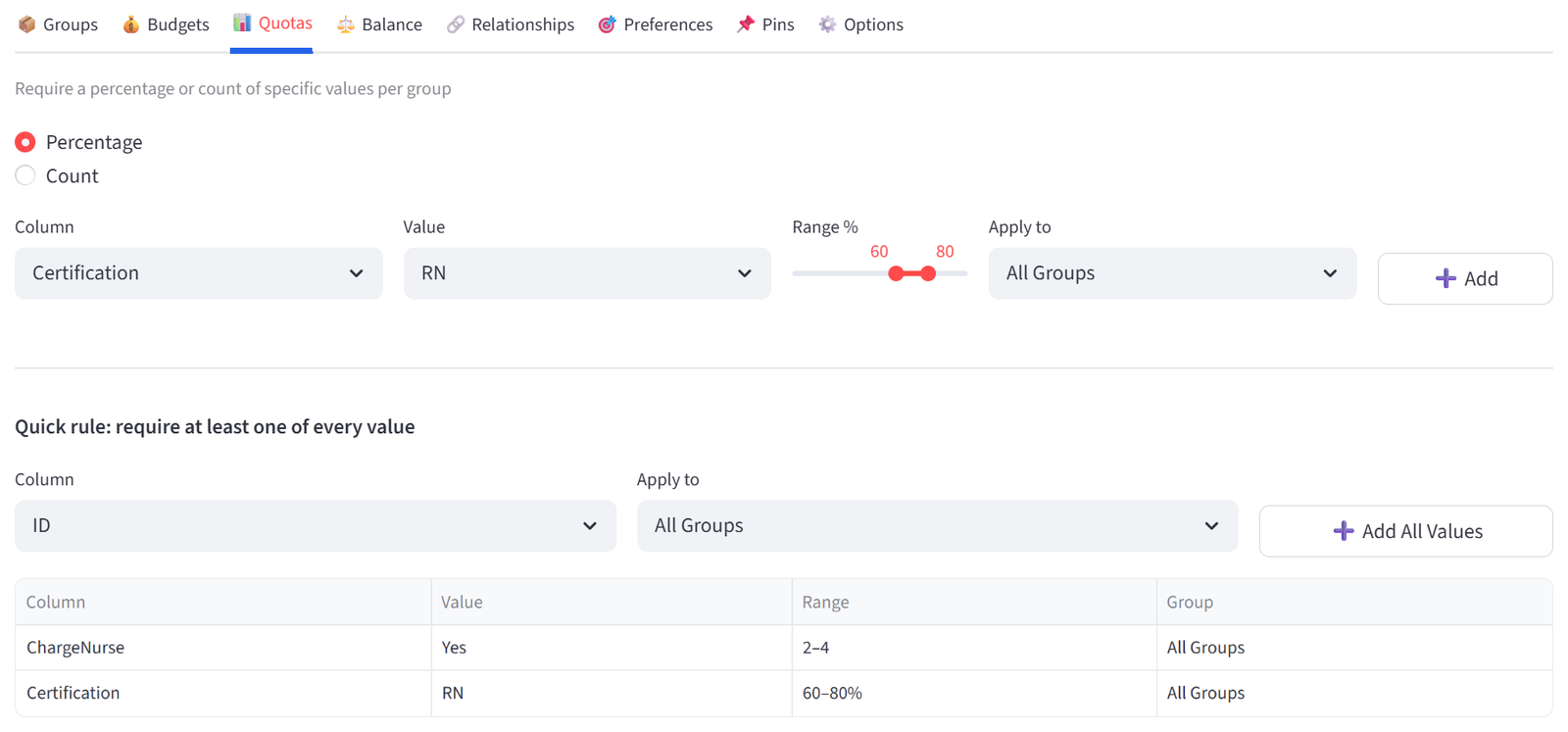
Tip: This ensures each shift has 2–4 Charge Nurses and 60–80% of staff are RNs.

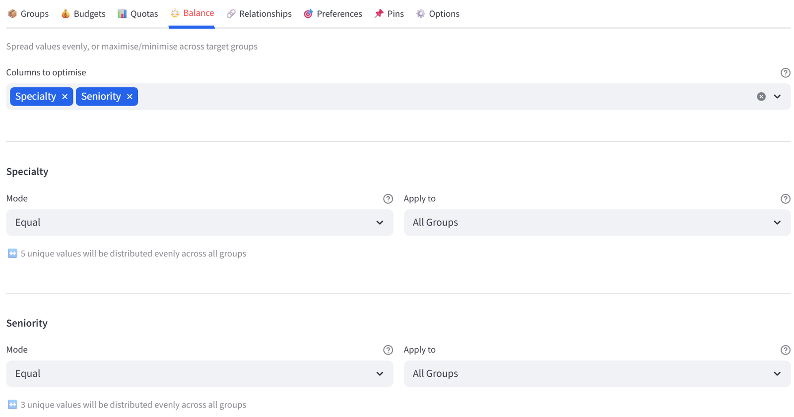
Step 5: Set Balance

Go to the Balance tab.
Select Specialty. Mode: Equal.
Select Seniority. Mode: Equal.

Step 6: Add Relationships — Incompatible Pairs

Go to Relationships tab.
Column: Incompatible, Type: KEEP_APART, Enforce: Required. Click Add.

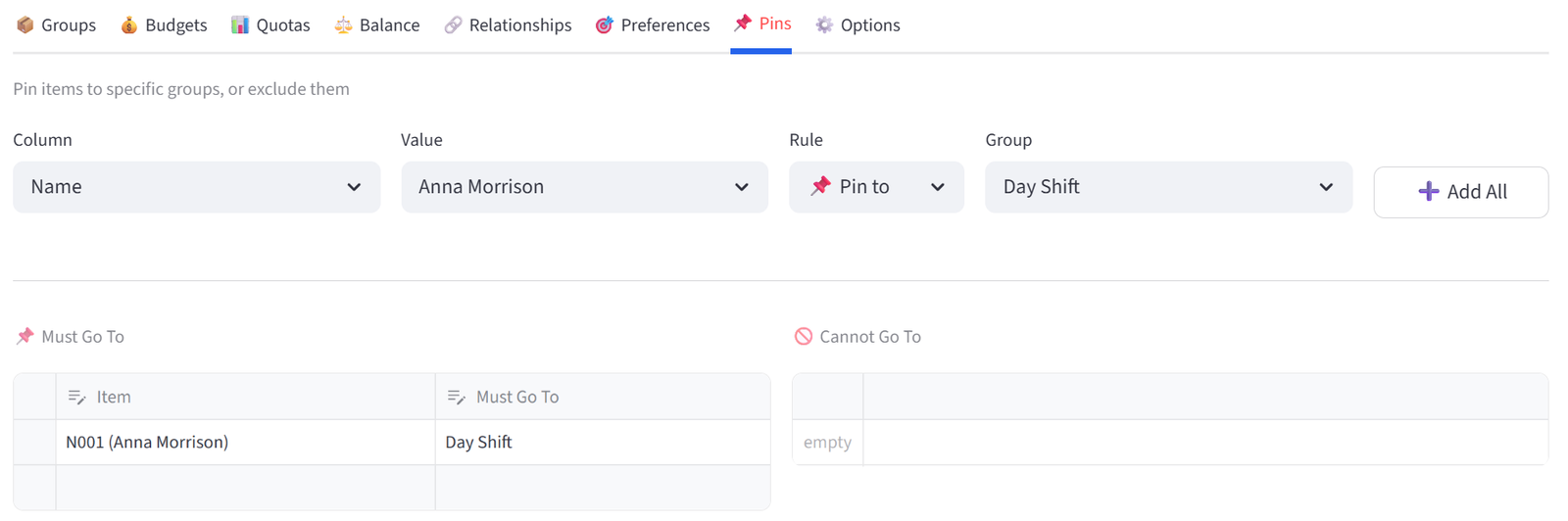
Step 7: Pin Head Nurse to Day Shift

Go to Pins tab.
Add Anna Morrison (N001) to Day Shift in the Must Go To editor.

Step 8: Run & Validate

Click Run Optimizer.
Check Validation: each shift has 2+ Charge Nurses, patient load hours are within budget, specialties are spread, incompatible pairs are separated.
Export for the scheduling coordinator.

Expected Outcome

Each shift has 9–11 nurses, 2–4 Charge Nurses, 60–80% RNs, and patient load hours between 140–180. Specialties and seniority levels are spread evenly. Incompatible pairs (Cooper/Ruiz, Li/Singh, Gomez/Lam) are on different shifts. Anna Morrison is on Day Shift.

This approach replaces what is typically a multi-hour manual scheduling process that frequently results in complaints about unfair distribution.

This example uses 30 nurses across 3 shifts. The same setup scales to 200+ staff across 6–12 shifts. Save the rules and reload them each roster cycle with updated staff availability data.

Appendix E: Sports — Under 8s Netball Grading

Scenario

Riverside Netball Club has 30 registered Under 8s players to grade into 4 teams. The club competes in a local league with a top division and a lower division. The grading coordinator needs: one strong team (Diamonds) for Division 1 matches, one development team (Rubies) for players who are newer or less experienced, and two middle teams (Opals and Sapphires) that are balanced evenly against each other for Division 2. Siblings must be kept together. Best friends should be kept together where possible. Parent coaches should be spread across teams.

The data includes 30 players with skill rating (0–100), preferred position (GS, GA, WA, C, WD, GD, GK), height, attendance rate, parent coach status, sibling links, best friend links, and years played. Skill ratings range from 40 (complete beginner) to 92 (experienced).

The Data

Save the following as netball_grading.csv:

30 rows, 10 columns. First 5 rows shown:

PlayerID	Name	SkillRating	Position	Height_cm	AttendanceRate	Parent_Coach	Siblings	BestFriend	YearsPlayed
N01	Ava Mitchell	92	GS	132	95	Yes		N02	2
N02	Chloe Tran	88	GA	128	90			N01	2
N03	Sophie Adams	85	WA	130	100			N04	2
N04	Ella Adams	83	GD	127	100			N03	2
N05	Mia Patel	90	C	135	95	Yes	N06		2

Full CSV file: netball_grading.csv

Step-by-Step Instructions

Step 1: Upload & Map

Upload netball_grading.csv.
Set Unique ID to PlayerID, Display Name to Name.
Import all columns.

Step 2: Set Terminology

In the sidebar, expand Terminology.
Change Item to ‘Player’, Group to ‘Team’, ID to ‘Player ID’. Click Apply.

Step 3: Configure Teams

Set Number of Teams to 4.
Rename to: Diamonds, Opals, Sapphires, Rubies.
Set Diamonds to Min 7 / Max 8.
Set Opals to Min 7 / Max 8.
Set Sapphires to Min 7 / Max 8.
Set Rubies to Min 7 / Max 8.
Add Tag ‘Middle’ to both Opals and Sapphires (type ‘Middle’ in each Tag cell).

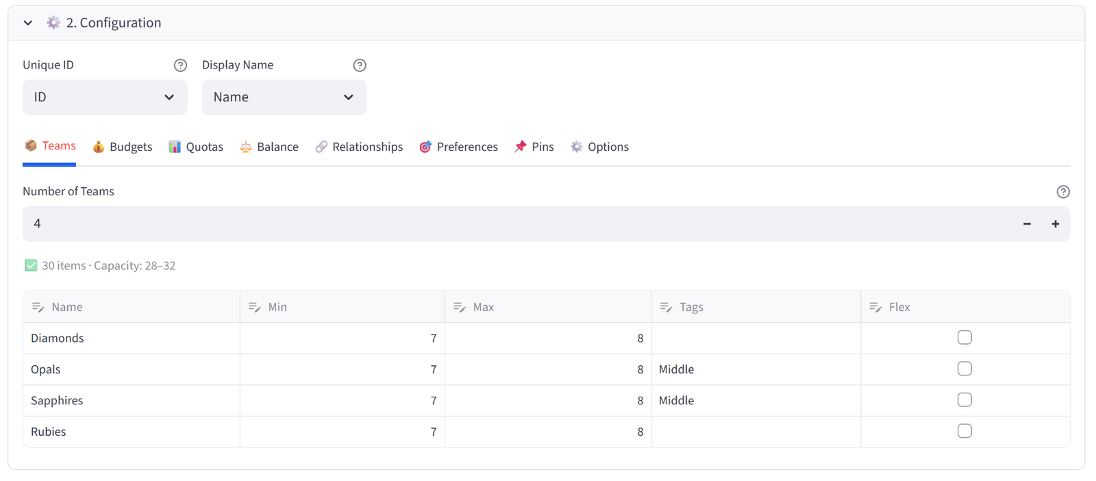
Tip: The ‘Middle’ tag lets you target Opals and Sapphires together in later rules.

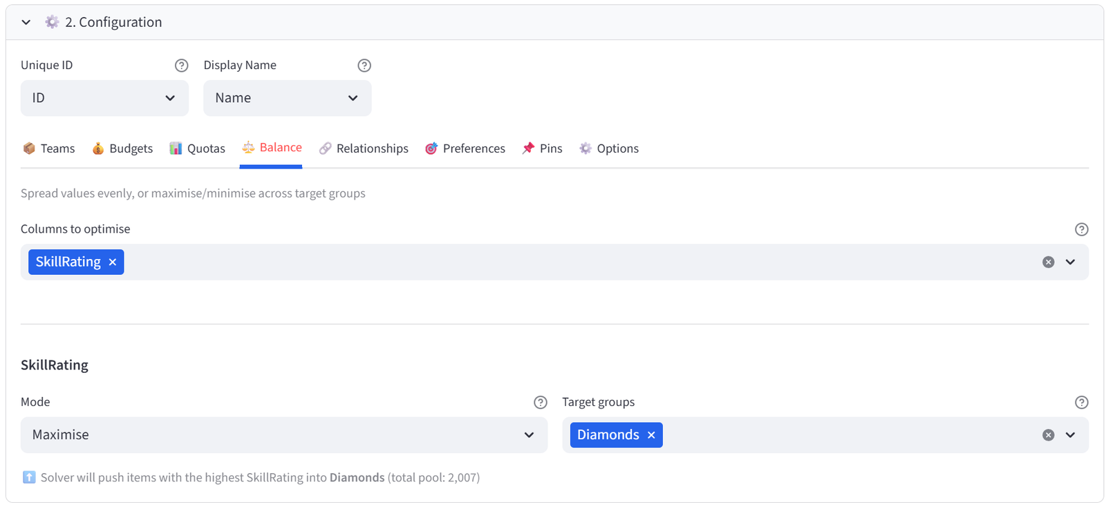
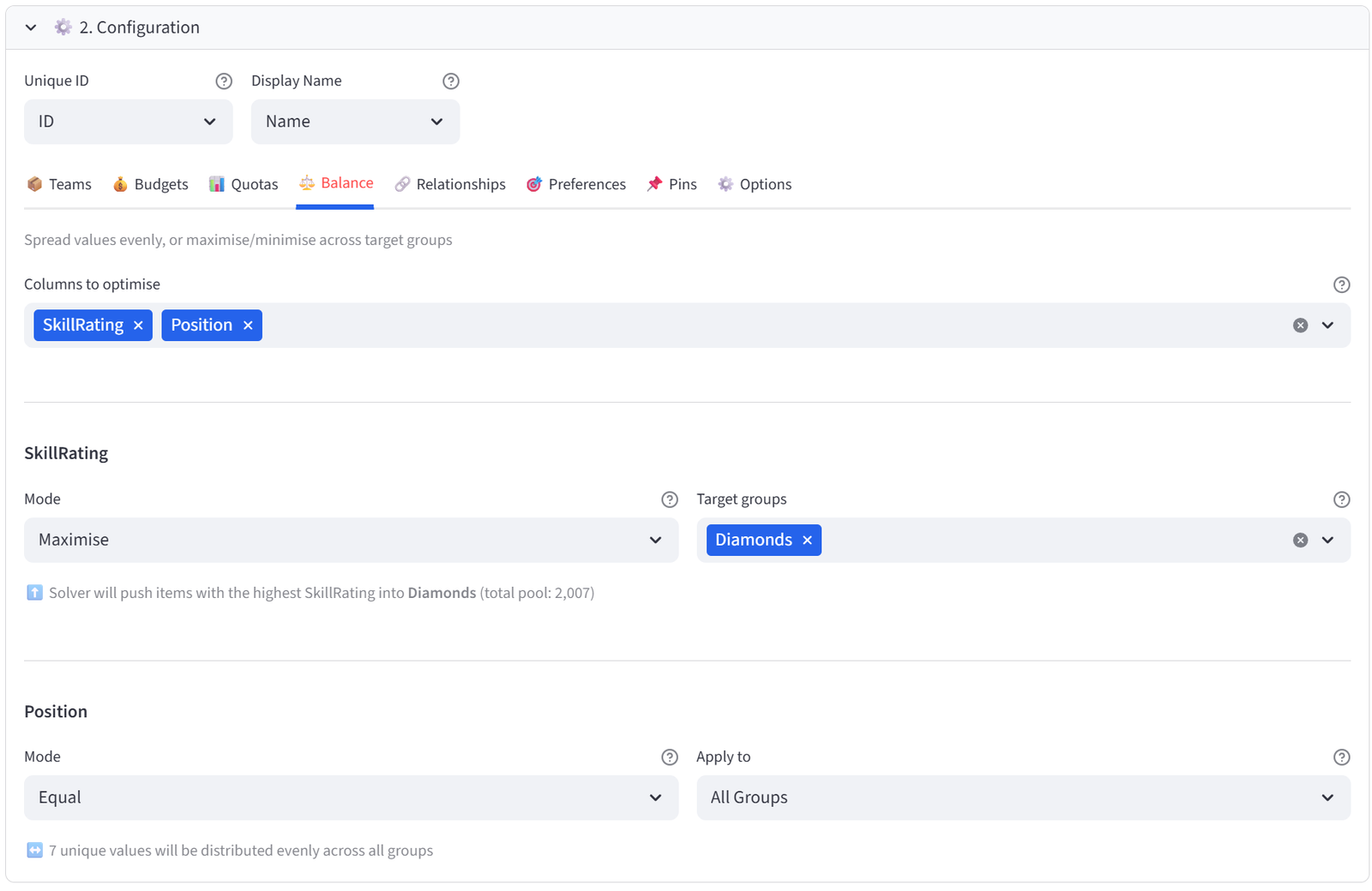
Step 4: Set Balance — Maximise Skill for Diamonds

Go to the Balance tab.
Select SkillRating from the multiselect.
Set Mode to Maximise. Set Target group(s) to Diamonds only.
This pushes the highest-rated players into Diamonds — the Division 1 team.

Step 5: Steer Beginners to Rubies via Preferences

Go to the Preferences tab.
Column: SkillRating, Operator: <, Value: 55, Target: Rubies, Strength: 85. Click Add.
Column: YearsPlayed, Operator: =, Value: 0, Target: Rubies, Strength: 70. Click Add.

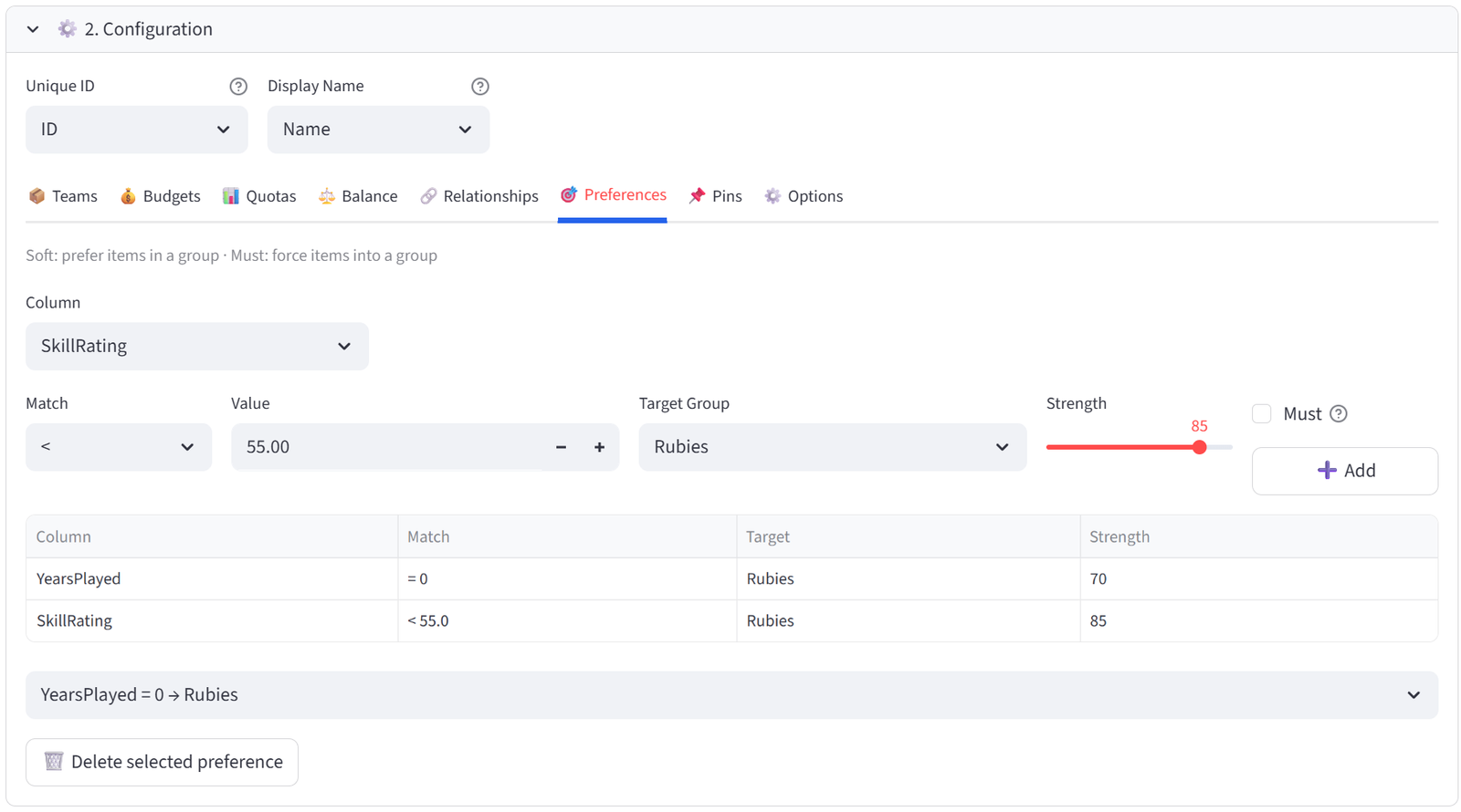
Tip: Players rated under 55 and those with zero years played are steered toward Rubies. Between the Maximise on Diamonds and these preferences, the middle-tier players naturally fill Opals and Sapphires.

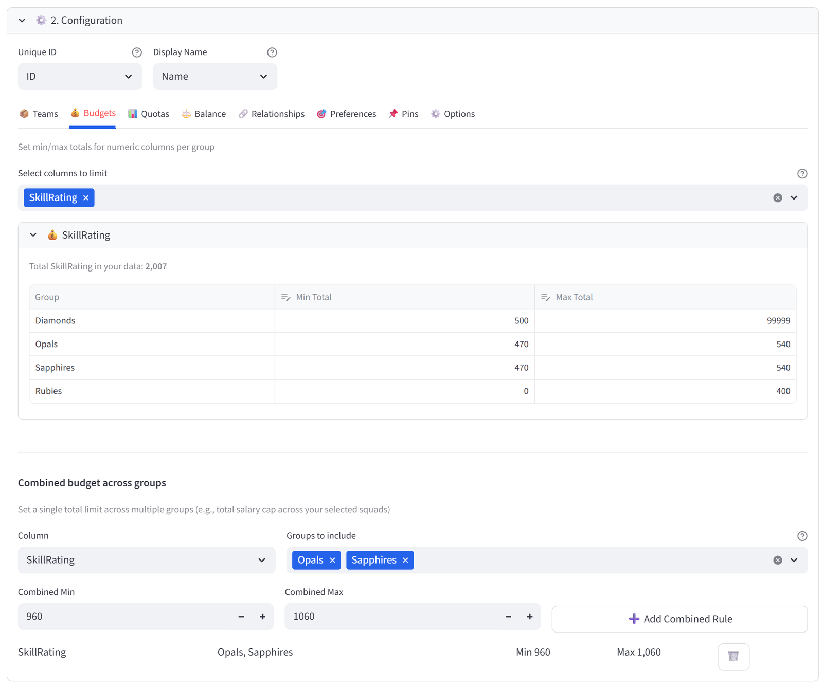
Step 6: Set Budget — Even Skill for Middle Teams

Go to the Budgets tab. Select SkillRating.
For Opals: set Min Total to 470, Max Total to 540.
For Sapphires: set Min Total to 470, Max Total to 540.
For Diamonds: set Min Total to 500, Max Total to 99999 (unconstrained upward).
For Rubies: set Min Total to 0, Max Total to 400.

Tip: The narrow 470–540 band forces Opals and Sapphires to be competitively even. Diamonds is uncapped so the solver can stack it. Rubies is capped low.

Step 7: Set Combined Budget — Shared Middle Total

In the Combined Budgets section below the individual budgets, click to add a combined budget.
Column: SkillRating, Groups: Opals + Sapphires, Min: 960, Max: 1060.

Tip: This combined constraint ensures the two middle teams share a fixed total pool of skill points. If Opals gets a slightly stronger player, Sapphires gets a slightly weaker one to compensate. This is the key to making them mirror teams.

Step 8: Set Quotas — Position Coverage and Parent Coaches

Go to Quotas tab. Use Count mode.
Column: Position, Value: GK, Min: 1, Max: 2. Group: All Teams. Click Add.
Column: Position, Value: GS, Min: 1, Max: 2. Group: All Teams. Click Add.
Column: Parent_Coach, Value: Yes, Min: 0, Max: 1. Group: All Teams. Click Add.

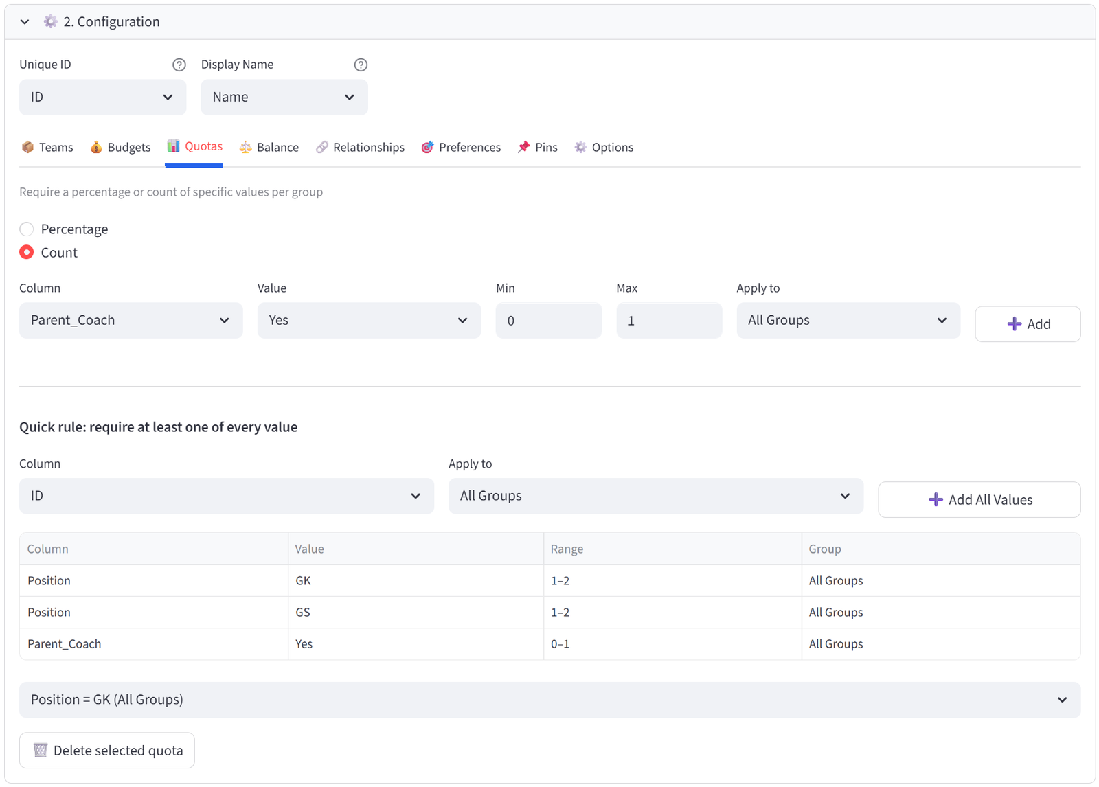
Tip: Every team needs at least one goalkeeper and one goal shooter. The parent coach quota (max 1 per team) spreads the 3 parent coaches across teams.

Step 9: Set Balance — Positions Across All Teams

Go back to Balance tab.
Select Position. Mode: Equal.
This spreads positions evenly so no team is all shooters or all defenders.

Step 10: Add Relationships — Siblings and Friends

Go to Relationships tab.
Column: Siblings, Type: KEEP_TOGETHER, Must Enforce: Tick (Required). Click Add.
Column: BestFriend, Type: KEEP_TOGETHER, Must Enforce: Untick (Preferred). Click Add.

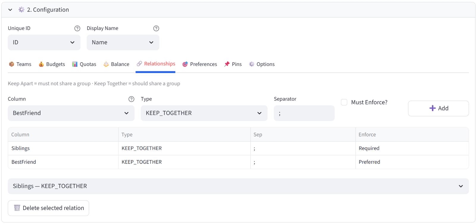
Tip: Siblings (Adams sisters N03/N04, Patel sisters N05/N06, Osei sisters N18/N19) must be together. Best friends are a soft preference that can be broken if needed.

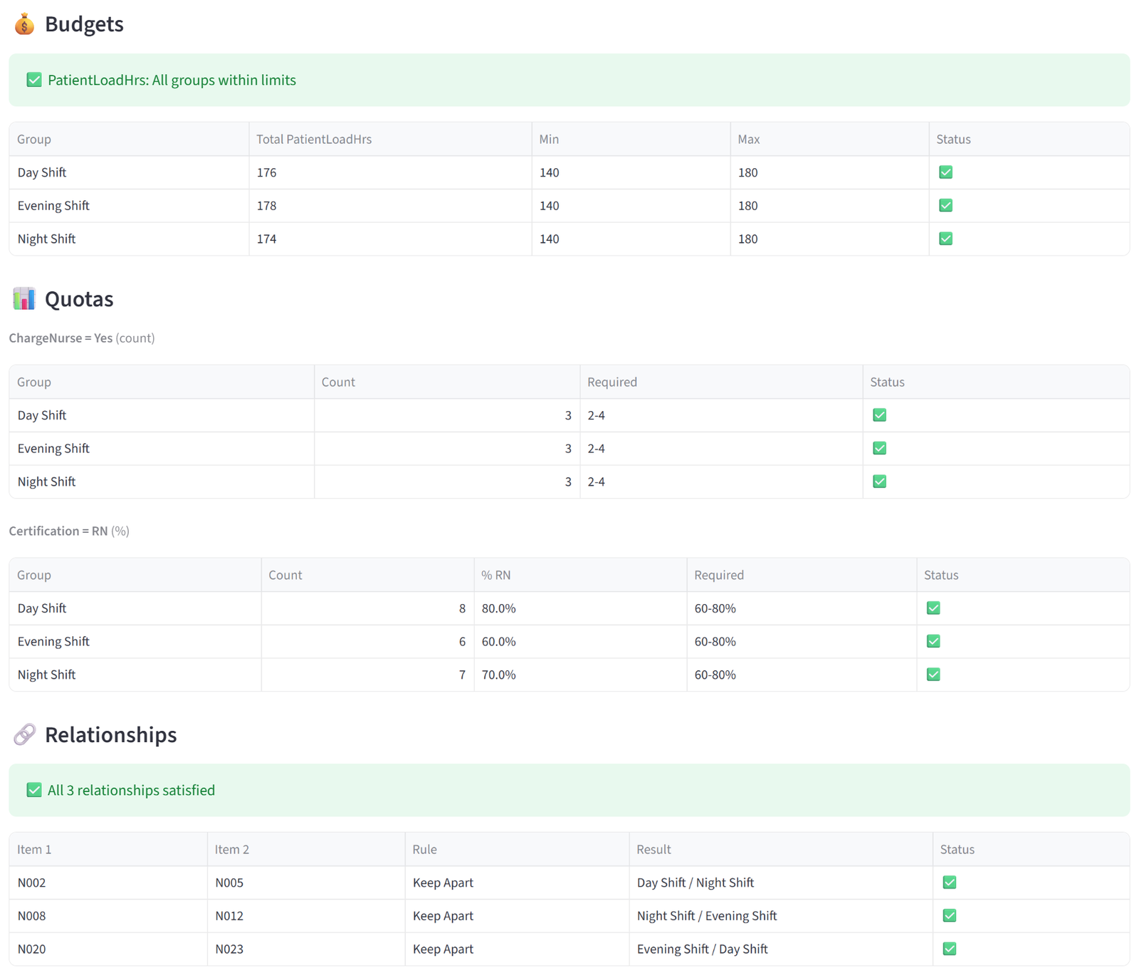
Step 11: Run & Validate

Click Run Optimizer.
Check Validation: Diamonds has the highest total skill, Rubies the lowest, Opals and Sapphires are within the 470–540 band and their combined total is 960–1060.
Review Rosters to confirm siblings are together.
Check Analytics to compare skill distributions across all four teams.
Export for the grading committee.

Expected Outcome

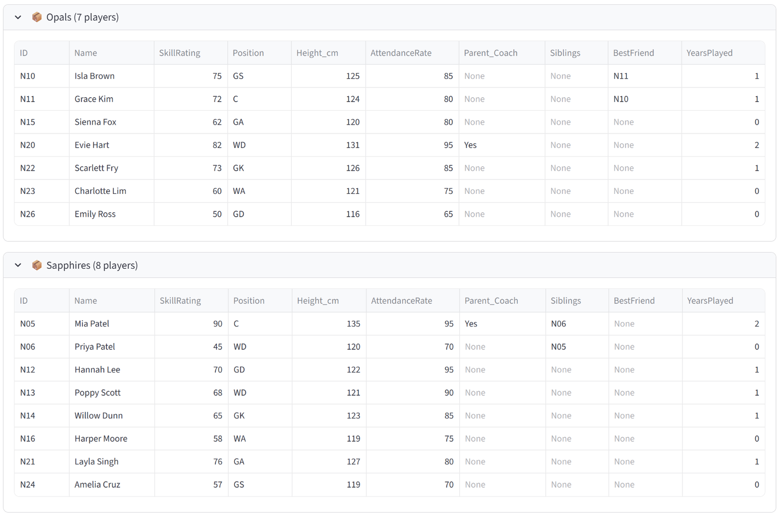
Diamonds (Division 1) has the 7–8 highest-rated players including Ava (92), Mia (90), Chloe (88), Lily (87), Sophie (85), and Olivia (84), with a combined skill rating above 550. Rubies (development) has the lowest-rated players with a combined rating under 400. Opals and Sapphires each sit in the 470–540 band, and their combined total falls within the 960–1060 range — making them competitively matched for Division 2.

Sibling pairs are together: Adams sisters on one team, Patel sisters together (even though Priya at 45 is weaker, she stays with Mia at 90 — this may pull one strong player out of Diamonds), Osei sisters together. Best friend pairs are together where possible. No team has more than one parent coach.

This demonstrates the key pattern of asymmetric grading: not all teams are equal. Maximise targets the strong team, Preferences steer the weak team, Budget bands lock the middle teams, and the Combined Budget ensures fairness between the pair. This is common in junior sports where you need a competitive top team and a supportive environment for beginners.

This example uses 30 players across 4 teams. Clubs with 60–120 registrations across 8–16 teams use the same configuration with more groups. Save the rules at the start of the season and reload them if late registrations require re-grading.

Appendix F: Government — Work Placement Scholarships

Scenario

The WA Department of Training administers 12 funded industry work placements for university students each year. There are 30 applicants competing for these spots. The program must balance merit (selecting the strongest applicants) with equity commitments: at least 3 placements for Indigenous students, at least 3 for regional students, representation across universities and fields of study, and a total stipend budget of $110,000.

This demonstrates the select/reject pattern: 12 applicants are selected into the ‘Awarded’ group, and the remaining 18 go into an ‘Applicant Pool’ (not selected). The solver maximises merit scores in the Awarded group while enforcing diversity quotas and a budget cap. This is fundamentally different from the other examples where all items are distributed — here, most items are rejected.

The data includes 30 applicants with university, field of study, GPA, merit score (composite of GPA, interview, portfolio), gender, Indigenous status, regional status, disability flag, stipend requirement, and optional employer preferences.

The Data

Save the following as work_placements.csv:

30 rows, 13 columns. First 5 rows shown:

AppID	Name	University	Field	GPA	MeritScore	Gender	Indigenous	Regional	DisabilityFlag	StipendReq
WP01	Aisha Kemp	UWA	Engineering	6.8	91	F	No	No	No	8000
WP02	Ben Tran	Curtin	Health Sciences	6.5	87	M	No	No	No	8000
WP03	Chelsea Maris	UWA	Engineering	6.2	83	F	Yes	Yes	No	10000
WP04	Daniel Yorke	Murdoch	Business	5.9	78	M	Yes	No	No	10000
WP05	Emma Stokes	ECU	Education	6.7	89	F	No	Yes	No	8000

Full CSV file: work_placements.csv

Step-by-Step Instructions

Step 1: Upload & Map

Upload work_placements.csv.
Set Unique ID to AppID, Display Name to Name.
Import all columns.

Step 2: Set Terminology

In the sidebar, expand Terminology.
Change Item to ‘Applicant’, Group to ‘Outcome’, ID to ‘Application ID’. Click Apply.

Step 3: Configure Groups — Awarded vs Pool

Set Number of Outcomes to 2.
Rename to: Awarded, Not Selected.
Set Awarded to Min 12 / Max 12 (exactly 12 placements).
Set Not Selected to Min 18 / Max 18.

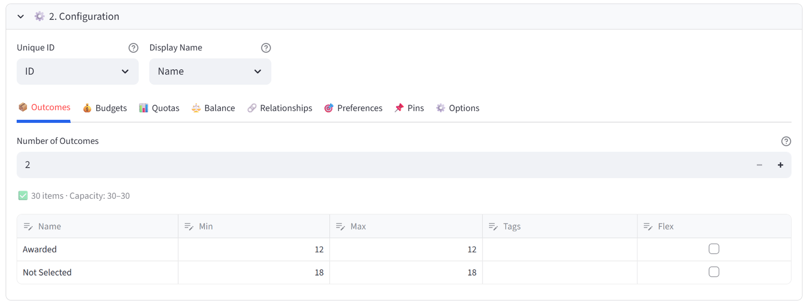
Tip: This is the key setup for select/reject: a fixed-size target group and a remainder group. The solver picks the best 12 while satisfying all constraints.

Step 4: Set Balance — Maximise Merit

Go to the Balance tab.
Select MeritScore from the multiselect.
Set Mode to Maximise. Set Target group to Awarded.

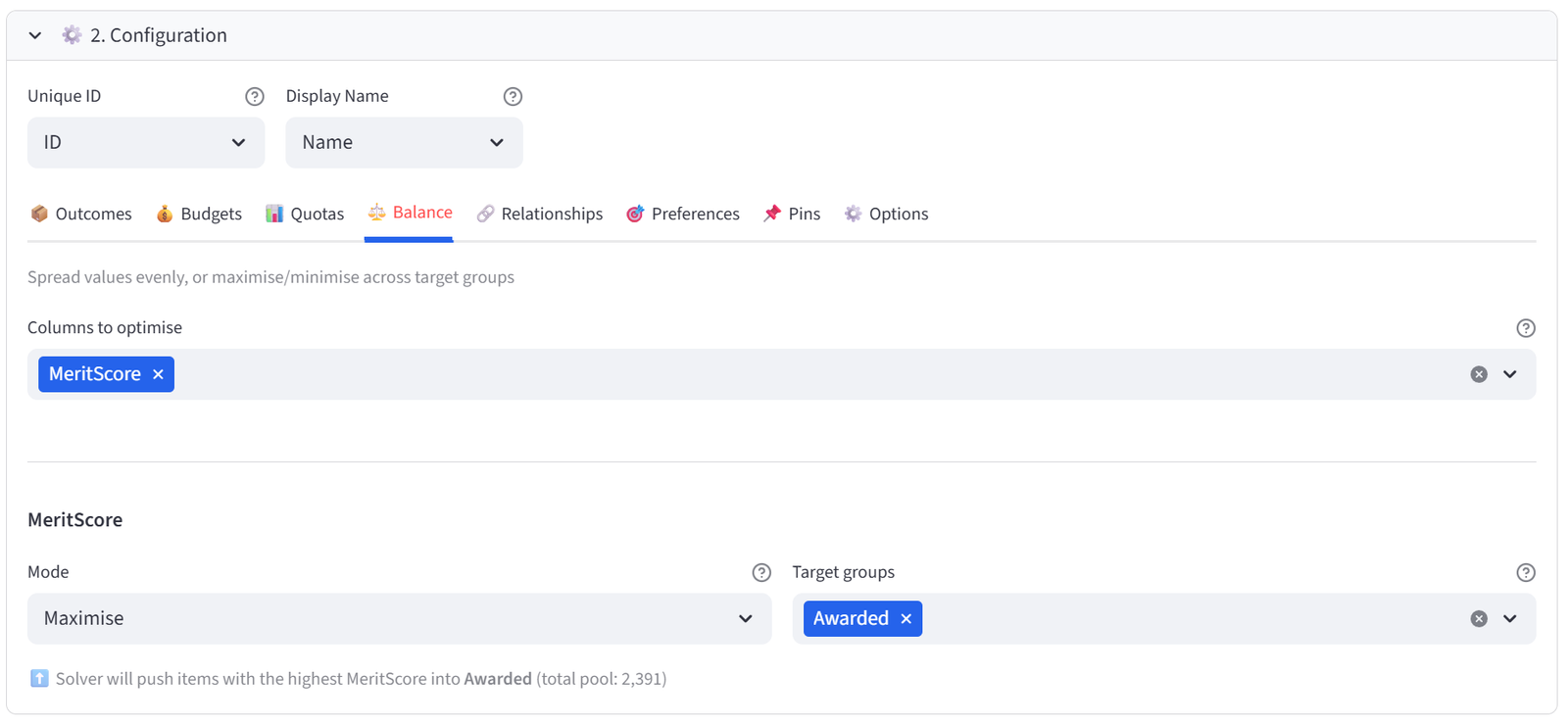
Tip: This is the core of the selection: the solver will try to place the highest-scoring applicants into Awarded. But the diversity quotas and budget below will override pure merit where needed.

Step 5: Set Budget — Stipend Cap

Go to the Budgets tab. Select StipendReq.
Set Awarded: Min Total to 0, Max Total to 110000.
Set Not Selected: leave unconstrained (Min 0, Max 9999999).

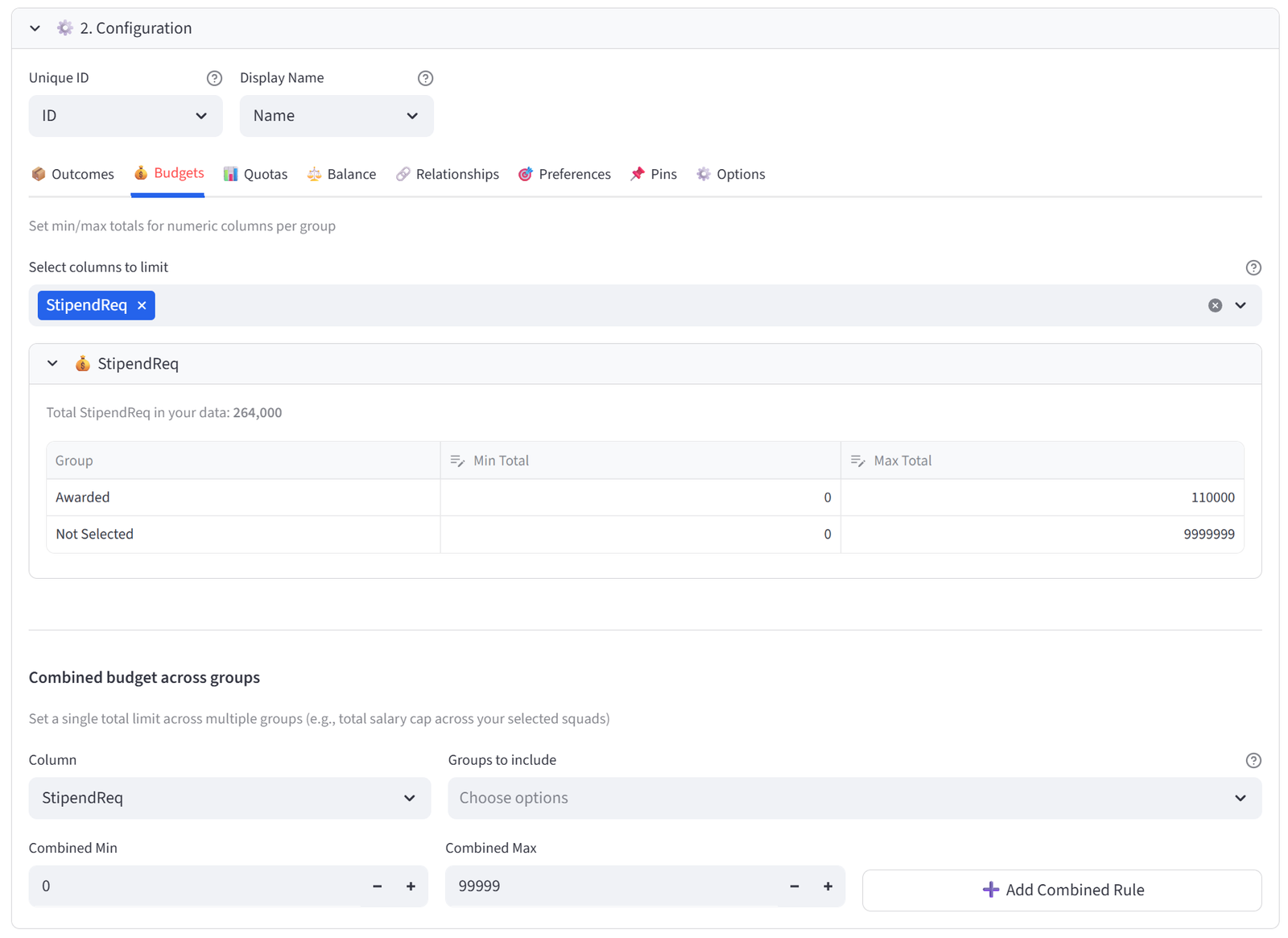
Tip: Indigenous and regional students have $10,000 stipends (higher support), others $8,000. With 12 spots and a $110,000 cap, the solver must balance the number of higher-stipend recipients. Pure merit might select 12 applicants costing $96,000–$120,000 — the budget forces trade-offs.

Step 6: Set Quotas — Indigenous Minimum

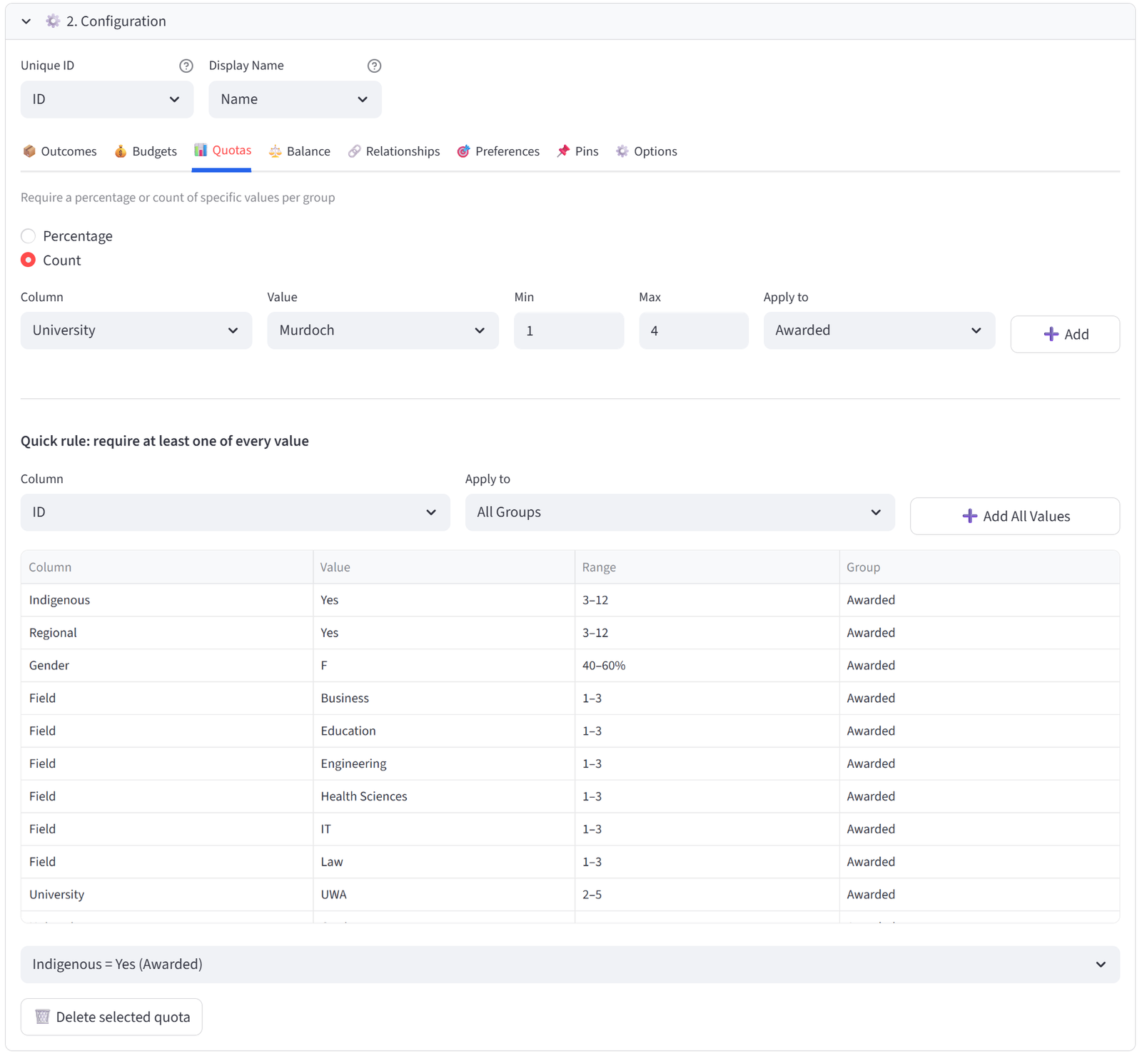
Go to Quotas tab. Use Count mode.
Column: Indigenous, Value: Yes, Min: 3, Max: 12. Group: Awarded. Click Add.

Tip: At least 3 of the 12 placements must go to Indigenous applicants. There are 8 Indigenous applicants in the pool, so this is achievable. The max of 12 means there is no upper cap — if merit supports more, the solver can select more.

Step 7: Set Quotas — Regional Minimum

Column: Regional, Value: Yes, Min: 3, Max: 12. Group: Awarded. Click Add.

Tip: At least 3 placements for regional students. There are 10 regional applicants.

Step 8: Set Quotas — Gender Balance

Switch to Percentage mode.
Column: Gender, Value: F, Min: 40, Max: 60. Group: Awarded. Click Add.

Step 9: Set Quotas — Field Diversity

Switch to Count mode.
Column: Field, Value: Engineering, Min: 1, Max: 3. Group: Awarded. Click Add.
Repeat for Health Sciences, IT, Law, Business, and Education (Min 1, Max 3 each).

Tip: This ensures the 12 placements span all 6 fields of study. No single field dominates.

Step 10: Set Quotas — University Spread

Column: University, Value: UWA, Min: 2, Max: 5. Group: Awarded. Click Add.
Repeat for Curtin, Murdoch, and ECU (Min 1, Max: 4 each).

Tip: Prevents all 12 placements going to one university.

Step 11: Run & Validate

Click Run Optimizer.
Check Validation: Awarded has exactly 12 applicants, at least 3 Indigenous, at least 3 Regional, 40–60% female, all 6 fields represented, stipend total ≤ $110,000.
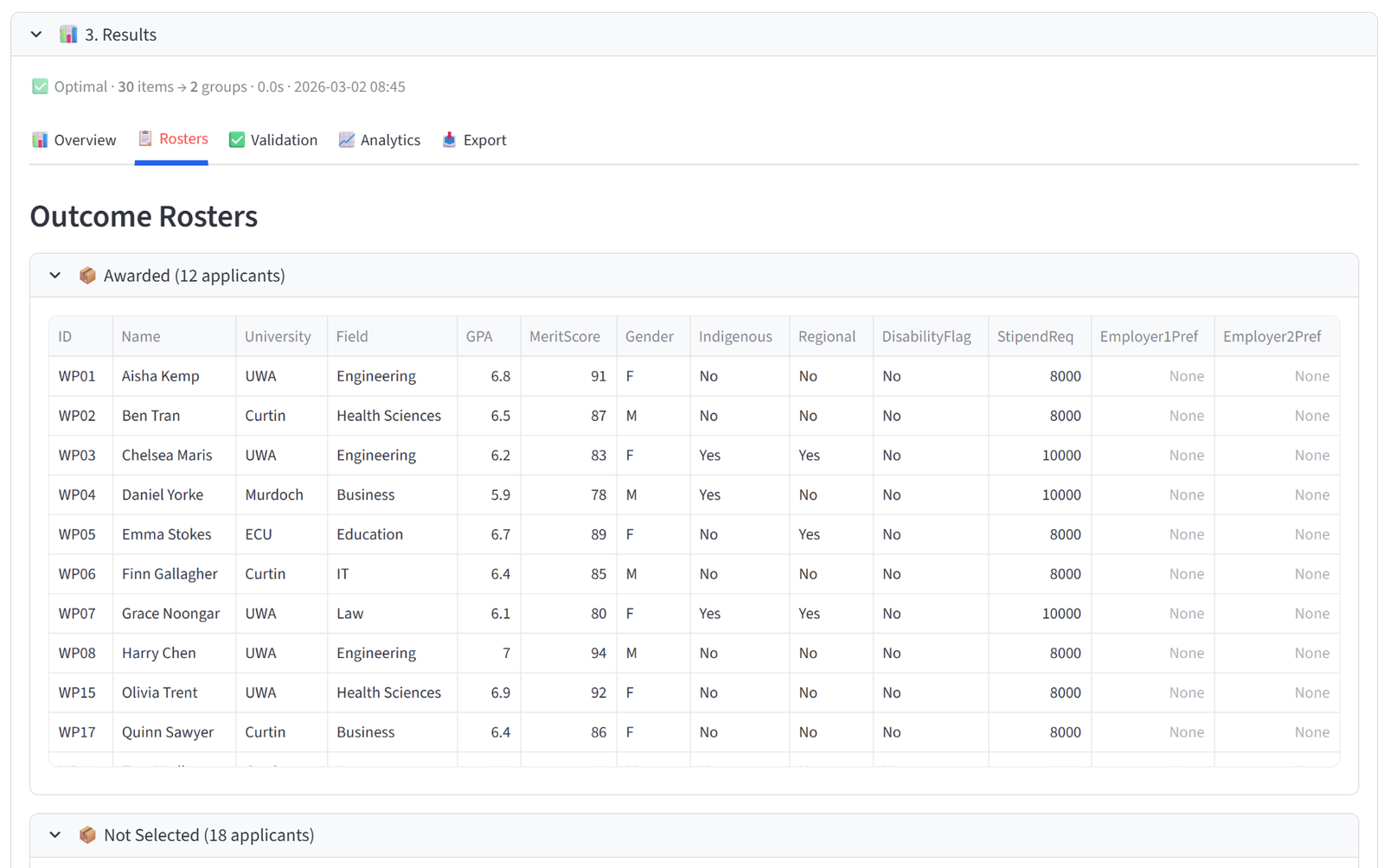
Review the Rosters tab: the Awarded group should contain the highest-scoring applicants that satisfy all equity constraints.
Compare the average MeritScore in Awarded vs Not Selected — there should be a clear gap.
Export the Awarded list for the selection panel.

Expected Outcome

Awarded contains 12 applicants with an average merit score of approximately 83–88 (the top end of the pool). Not Selected contains 18 applicants with lower average scores. The total stipend is at or just under $110,000.

At least 3 Indigenous students and 3 regional students are included. Gender is 40–60% female. All 6 fields of study are represented. Multiple universities contribute. Some high-scoring applicants may miss out if they would break a diversity quota or push the stipend over budget.

This is the select/reject pattern: not every applicant gets placed. The solver maximises merit in the Awarded group while enforcing equity and budget constraints. The Not Selected group is the reject pool. This pattern applies to any competitive selection: grants, scholarships, internships, awards shortlisting, or program admissions.

This example uses 30 applicants for 12 spots. The same approach scales to hundreds of applicants — for example, 500 grant applications for 40 funded positions. The solver handles the combinatorial complexity instantly. Save the rules and reuse them each funding round with a fresh applicant list.

Appendix G: Real Estate — Tenant Allocation

Scenario

Harbour Point has 28 commercial tenants applying for space in 4 buildings plus a waitlist. Buildings have different capacities. Harbour Tower and Marina West share a site with only 800m² of parking between them, demonstrated using a combined budget. There are more tenants than spaces, so 3 buildings hold 6 each, 1 holds 5, and the remainder go on a Waitlist group.

This demonstrates three patterns not shown in other examples: (1) a reject/overflow group for items that don’t fit, (2) a combined budget across two groups sharing a resource, and (3) targeting budgets and preferences at specific groups while letting the waitlist absorb the rest.

The data includes 28 tenants with sector, lease tier, annual revenue, square metre needs, lease years, floor preference, conflicts, and parking needs.

The Data

Save the following as tenant_allocation.csv:

28 rows, 10 columns. First 5 rows shown:

TenantID	Company	Sector	LeaseTier	AnnualRevenue	SqMetres	LeaseYears	FloorPref	Conflicts	NeedsParking
T001	Apex Legal	Professional	Premium	320000	280	5	High		Yes
T002	ByteForce	Tech	Premium	450000	350	3	High	T008	Yes
T003	ClearView Finance	Finance	Premium	380000	300	5	High		Yes
T004	DataStream	Tech	Standard	180000	200	3	Mid		Yes
T005	EcoGreen Solutions	Environment	Standard	95000	120	3	Low		No

Full CSV file: tenant_allocation.csv

Step-by-Step Instructions

Step 1: Upload & Map

Upload tenant_allocation.csv.
Set Unique ID to TenantID, Display Name to Company.
Import all columns.

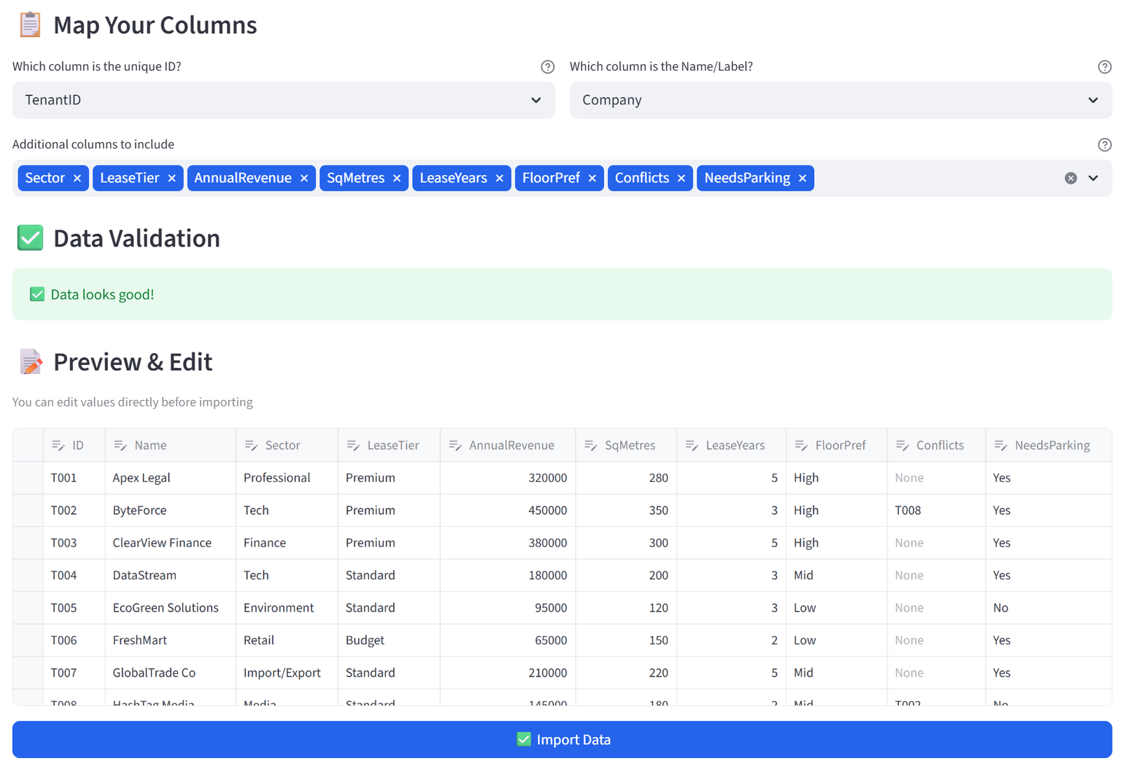
Step 2: Set Terminology

Change Item to ‘Tenant’, Group to ‘Building’, ID to ‘Tenant ID’.

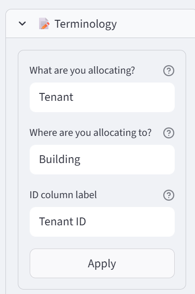
Step 3: Configure Buildings + Waitlist

Set Number of Buildings to 5.
Rename to: Harbour Tower, Marina West, Pier One, Dock View, Waitlist.
Set Harbour Tower to Min 6 / Max 7.
Set Marina West, Pier One, Dock View to Min 5 / Max 6.
Set Waitlist to Min 0 / Max 10. Tick the Flex checkbox for Waitlist.
Add Tag ‘SharedSite’ to Harbour Tower and Marina West.
Add Tag ‘Active’ to Harbour Tower, Marina West, Pier One, and Dock View.

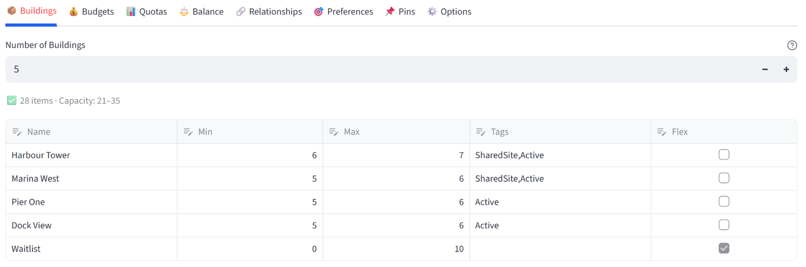
Tip: The Waitlist group absorbs tenants that don’t fit. Flex means the solver can put more in if needed. Tags let you target rules at the 4 real buildings or the 2 shared-site buildings.

Step 4: Set Budget — Revenue Floor for Active Buildings

Go to Budgets tab. Select AnnualRevenue.
Set Min Total to 500000 for Harbour Tower, Marina West, Pier One, Dock View.
Set Max Total to 1500000 for Harbour Tower, 900000 for others.
Set Waitlist: Min Total to 0, Max Total to 9999999 (no limit).

Tip: The revenue floor ensures each real building is commercially viable. The Waitlist has no revenue constraint.

Step 5: Set Combined Budget — Shared Parking

Still in the Budgets tab, scroll to the Combined Budgets section below the per-group table.
Click to add a combined budget.
Column: SqMetres. Groups: select Harbour Tower and Marina West.
Set Combined Max to 2000.
Leave Combined Min at 0.

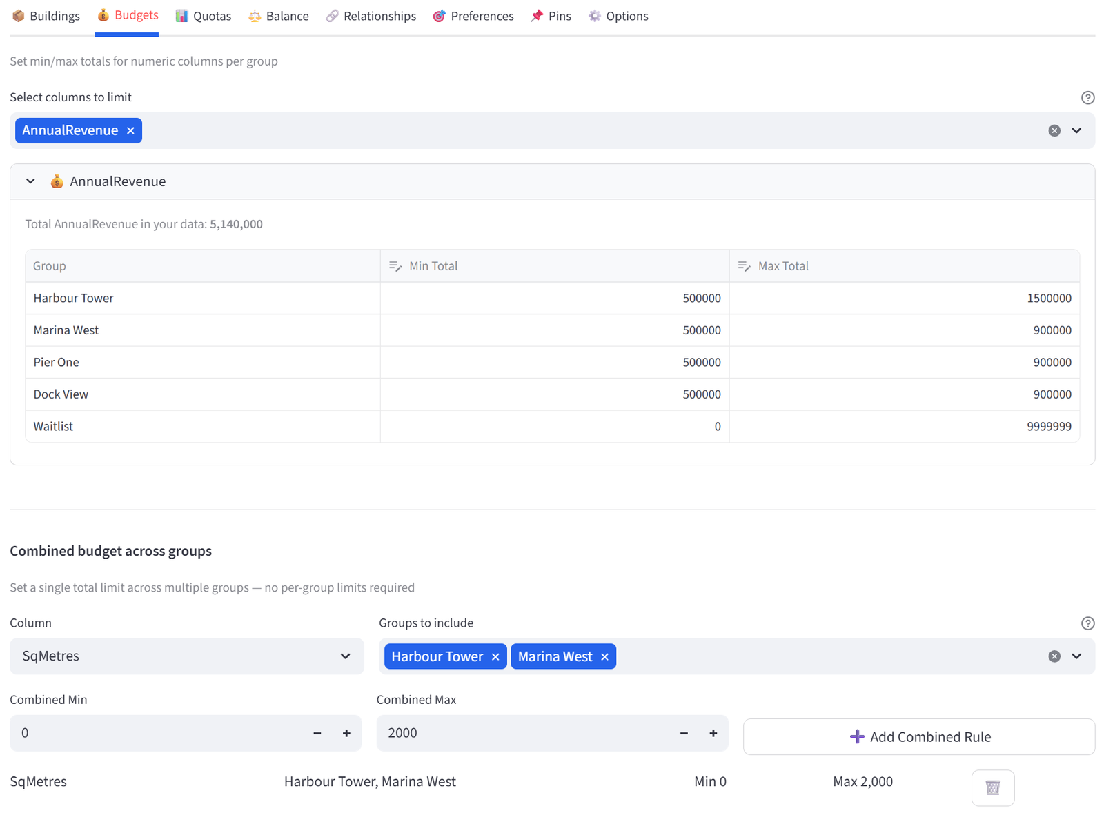
Tip: Harbour Tower and Marina West share a site with limited parking infrastructure. Their combined tenant square metre footprint (which drives parking demand) cannot exceed 2,000m². With 11–13 tenants across both buildings, this forces the solver to favour smaller tenants for these two buildings and push larger-footprint tenants to Pier One, Dock View, or the Waitlist.

Step 6: Set Balance — Lease Tier (Active Buildings Only)

Go to Balance tab. Select LeaseTier. Mode: Equal.
In the ‘Apply to’ dropdown, select Tag: Active.
This spreads Premium, Standard, and Budget tenants evenly across the four real buildings only. The Waitlist is excluded from balancing because we did not previously Tag it ‘Active’, so it can absorb whatever mix of tenants doesn’t fit.

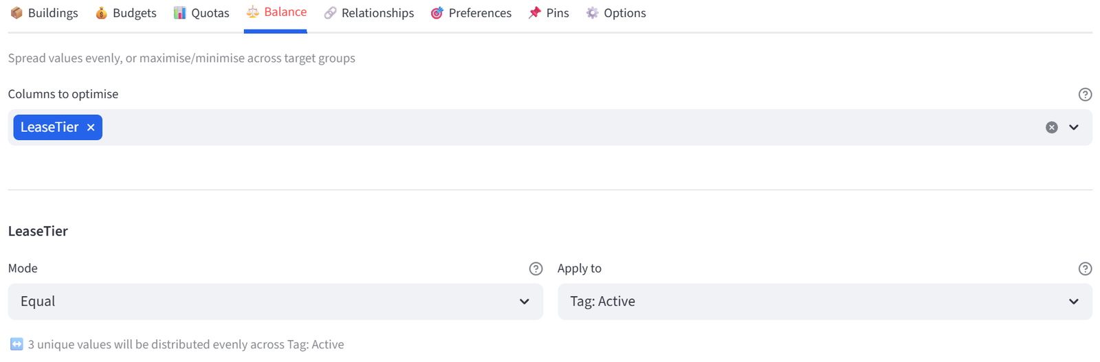
Step 7: Add Preference — Premium to Harbour Tower, Budget to Waitlist

Go to Preferences tab.
Column: LeaseTier, Operator: =, Value: Premium, Target: Harbour Tower, Strength: 70. Click Add.
Column: LeaseTier, Operator: =, Value: Budget, Target: Waitlist, Strength: 50. Click Add.
Column: NeedsParking, Operator: =, Value: No, Target: Harbour Tower, Strength: 40. Click Add.

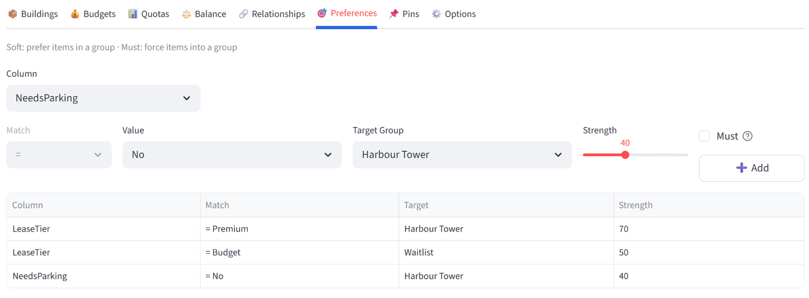
Tip: Premium tenants are pulled toward the flagship. Budget tenants are gently pushed to the waitlist (but only as a soft preference — if they meet the revenue requirements, they can still be placed). Tenants not needing parking are preferred for Harbour Tower to reduce pressure on the shared parking constraint.

Step 8: Add Relationships — Conflicts

Go to Relationships tab.
Column: Conflicts, Type: KEEP_APART, Enforce: Required. Click Add.

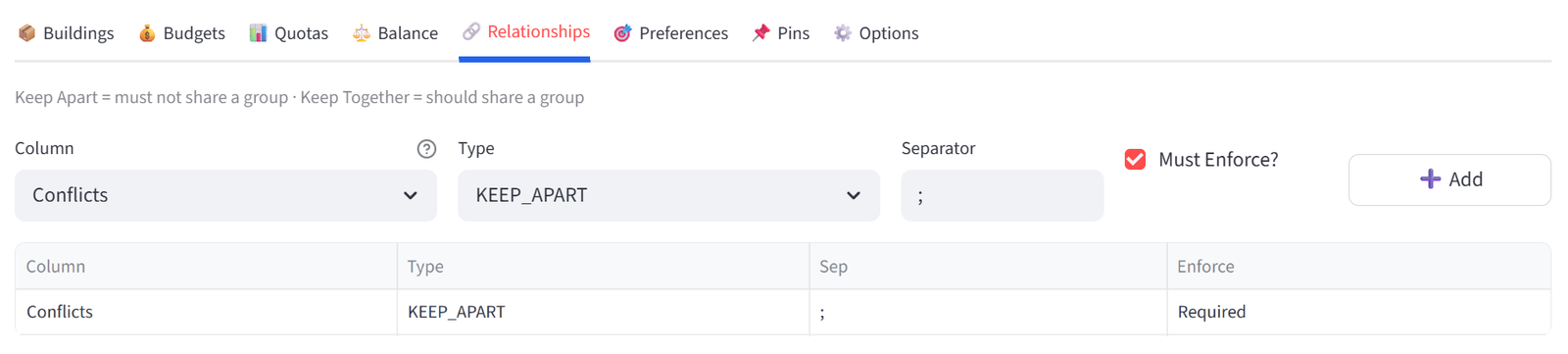
Step 9: Run & Validate

Click Run Optimizer.
Check: each active building meets $500K revenue, Harbour Tower + Marina West combined SqMetres ≤ 2000, ByteForce and HashTag Media are in different buildings.
Review the Waitlist group — it should contain tenants that didn’t fit the constraints.
Export the allocation report for the leasing team.

Expected Outcome

Harbour Tower, Marina West, Pier One, and Dock View each have 5–7 tenants and exceed $500K in annual revenue. The Waitlist holds the tenants that couldn’t fit the constraints. Harbour Tower and Marina West’s combined square metre footprint stays under 2,000m².

Premium tenants cluster in Harbour Tower and the other active buildings. Some Budget tenants land on the Waitlist. ByteForce (T002) and HashTag Media (T008) are in different buildings.

This example demonstrates three important patterns: (1) the Waitlist as a reject/overflow group — not every item has to be placed in a ‘real’ group, (2) combined budgets for shared resources across building pairs, and (3) preferences that steer lower-priority items toward the overflow group while ensuring high-value items get placed. The same setup scales to 100+ tenants across 10–20 buildings with multiple shared-site pairs.

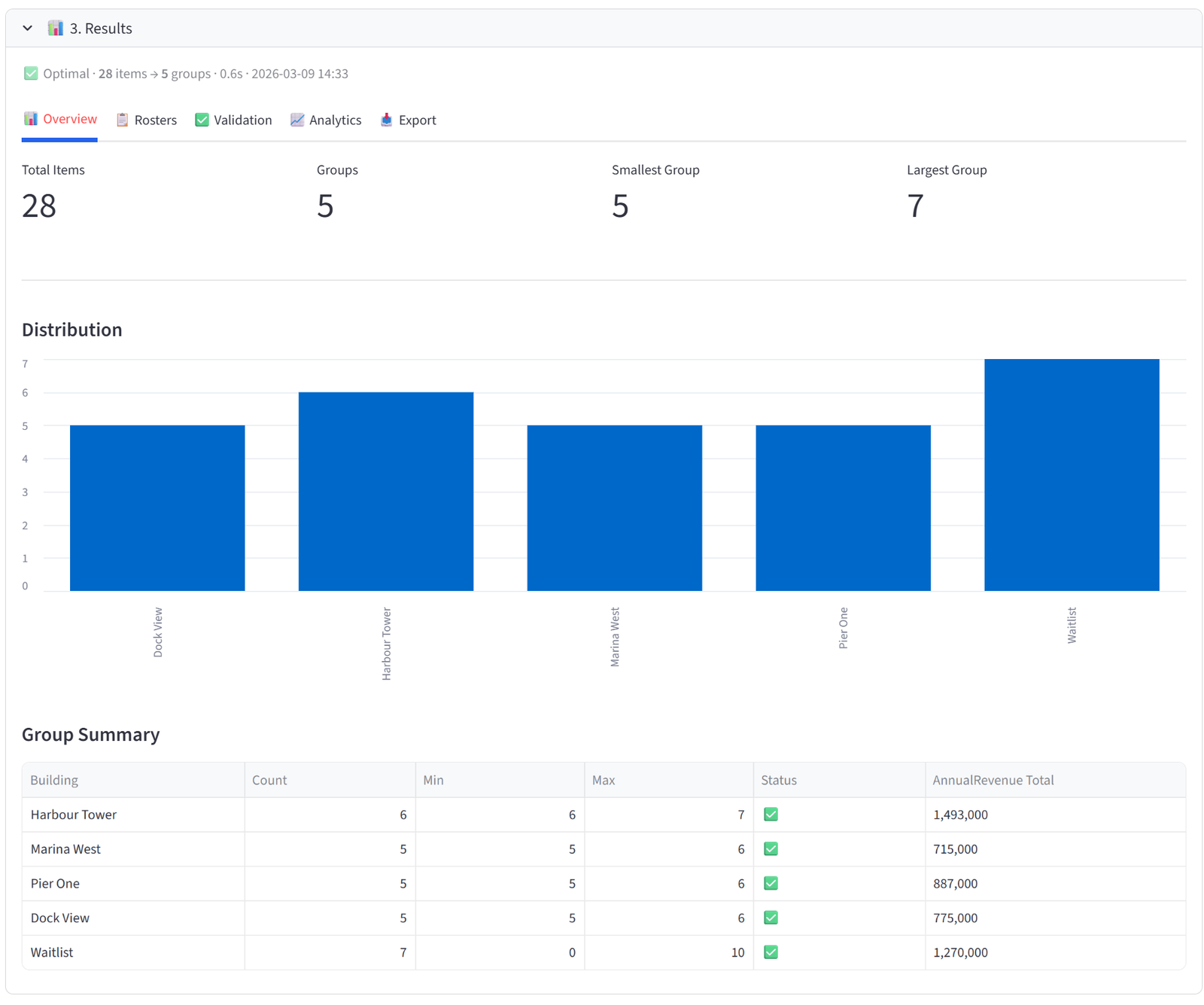
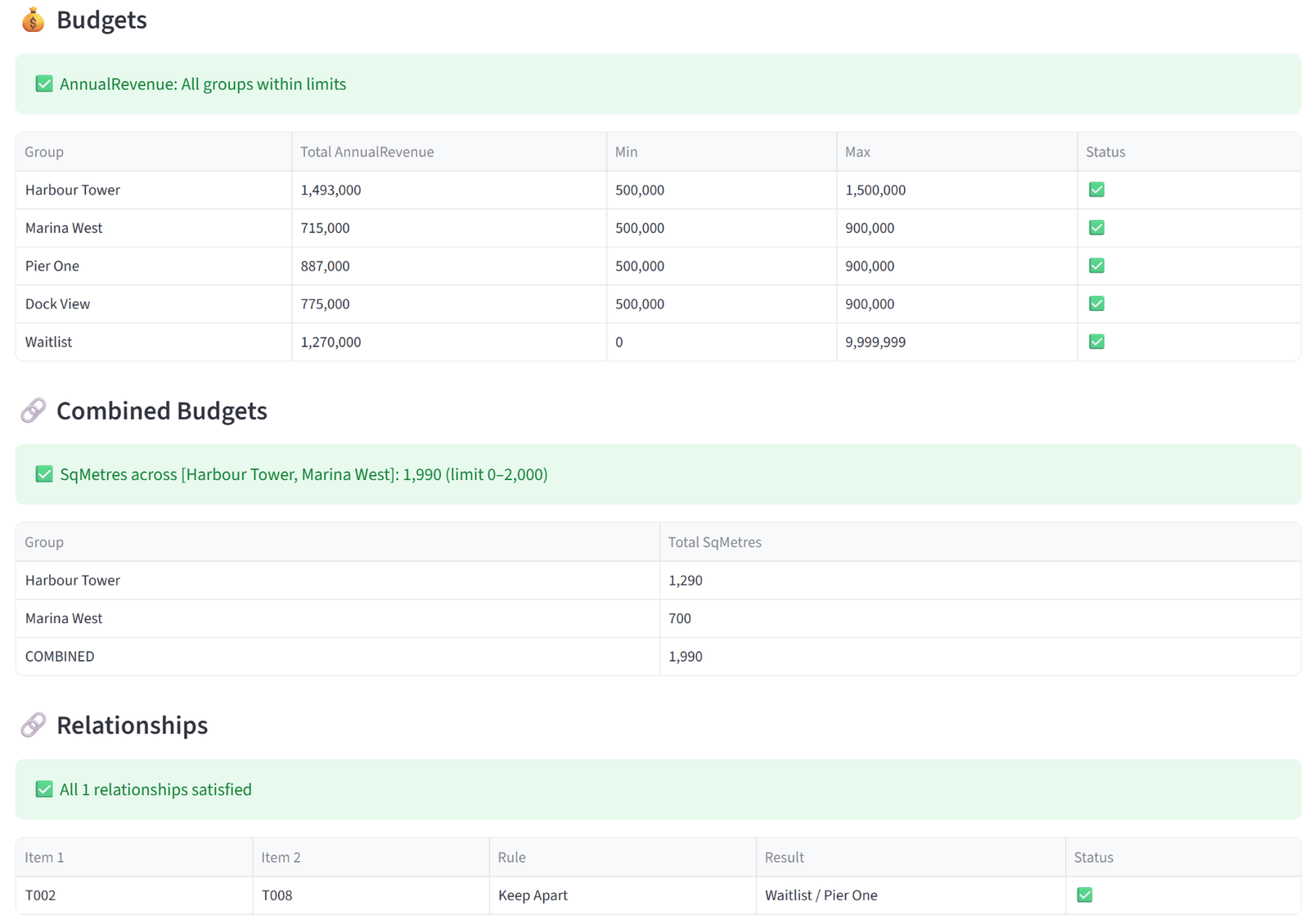
Appendix H: Manufacturing — Production Line Balancing

Scenario

Precision Engineering runs 4 production lines with 24 operators. Each operator has primary and secondary certifications (CNC, Welding, Assembly, Quality), a certification level (1–3), years of experience, shift preference, and safety score. Lines need balanced certification coverage and total experience years within a range.

The data includes 24 operators with certifications, level, experience, shift preference, mentor flag, and safety score.

The Data

Save the following as production_line.csv:

24 rows, 9 columns. First 5 rows shown:

OperatorID	Name	PrimaryCert	SecondCert	CertLevel	ExpYears	ShiftPref	Mentor	SafetyScore
OP01	Alan Ford	CNC	Welding	Level 3	18	Day		98
OP02	Beth Moore	Assembly	Quality	Level 2	8	Day		88
OP03	Carl Dunn	CNC	Assembly	Level 3	15	Day		95
OP04	Diana Voss	Welding	CNC	Level 2	7	Night		85
OP05	Ed Park	Assembly	Welding	Level 1	2	Day		72

Full CSV file: production_line.csv

Step-by-Step Instructions

Step 1: Upload & Map

Upload production_line.csv.
Set Unique ID to OperatorID, Display Name to Name.
Import all columns.

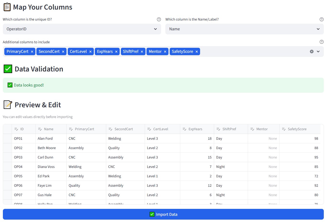
Step 2: Configure Lines

Set Number of Groups to 4.
Rename: Line Alpha, Line Beta, Line Gamma, Line Delta.
Set each to Min 5 / Max 7.

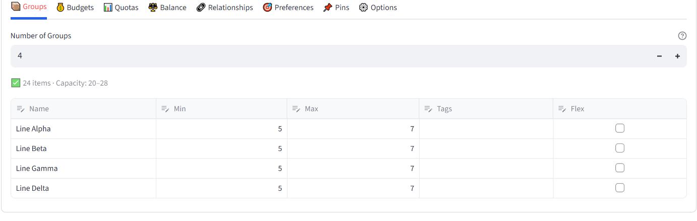
Step 3: Set Budget — Experience Years

Go to Budgets tab. Select ExpYears.
Set Min Total to 30, Max Total to 55 for each line.

Tip: Total experience across all operators is ~192 years. With 4 lines at 30–55 each (120–220 range), the solver has room to balance.

Step 4: Set Budget — Safety Score

Whilst still on Budgets tab. Select SafetyScore.
Set Min Total to 460, Max Total to 560 for each line.

Tip: This prevents any line from having all low-safety-score rookies.

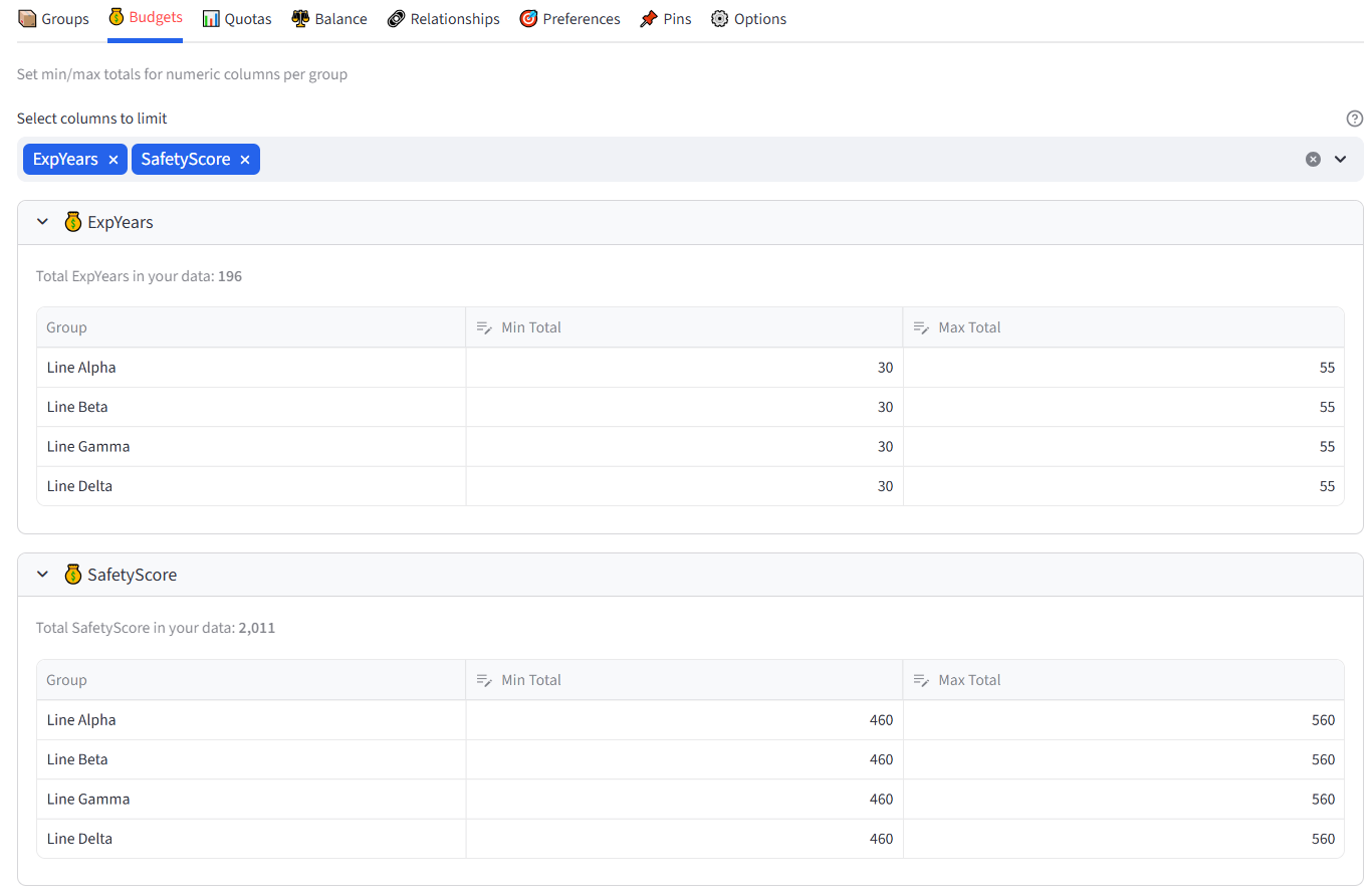
Step 5: Set Quotas — Certification Levels

Go to Quotas tab. Use Count mode.
Column: CertLevel, Value: Level 3, Min: 2, Max: 3. Group: All Groups. Click Add.
Column: CertLevel, Value: Level 1, Min: 1, Max: 3. Group: All Groups. Click Add.

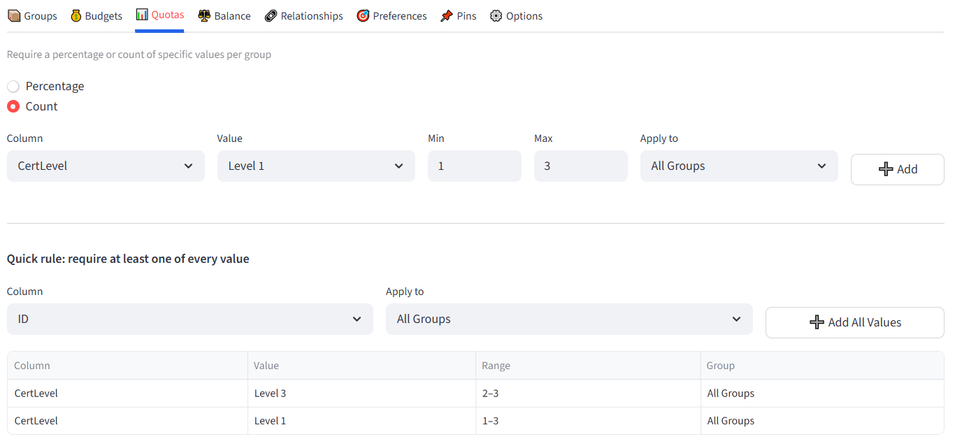
Tip: This ensures each line has experienced leaders (Level 3) and some junior operators (Level 1) for training.

Step 6: Set Balance — Primary Certification

Go to Balance tab.
Select PrimaryCert. Mode: Equal. Apply to: All Groups.
This distributes CNC, Welding, Assembly, and Quality operators across all lines.

Step 7: Add Balance — Shift Preference

Also select ShiftPref in the Balance tab. Mode: Equal. Apply to: All Groups.
This ensures Day and Night preference operators are spread evenly.

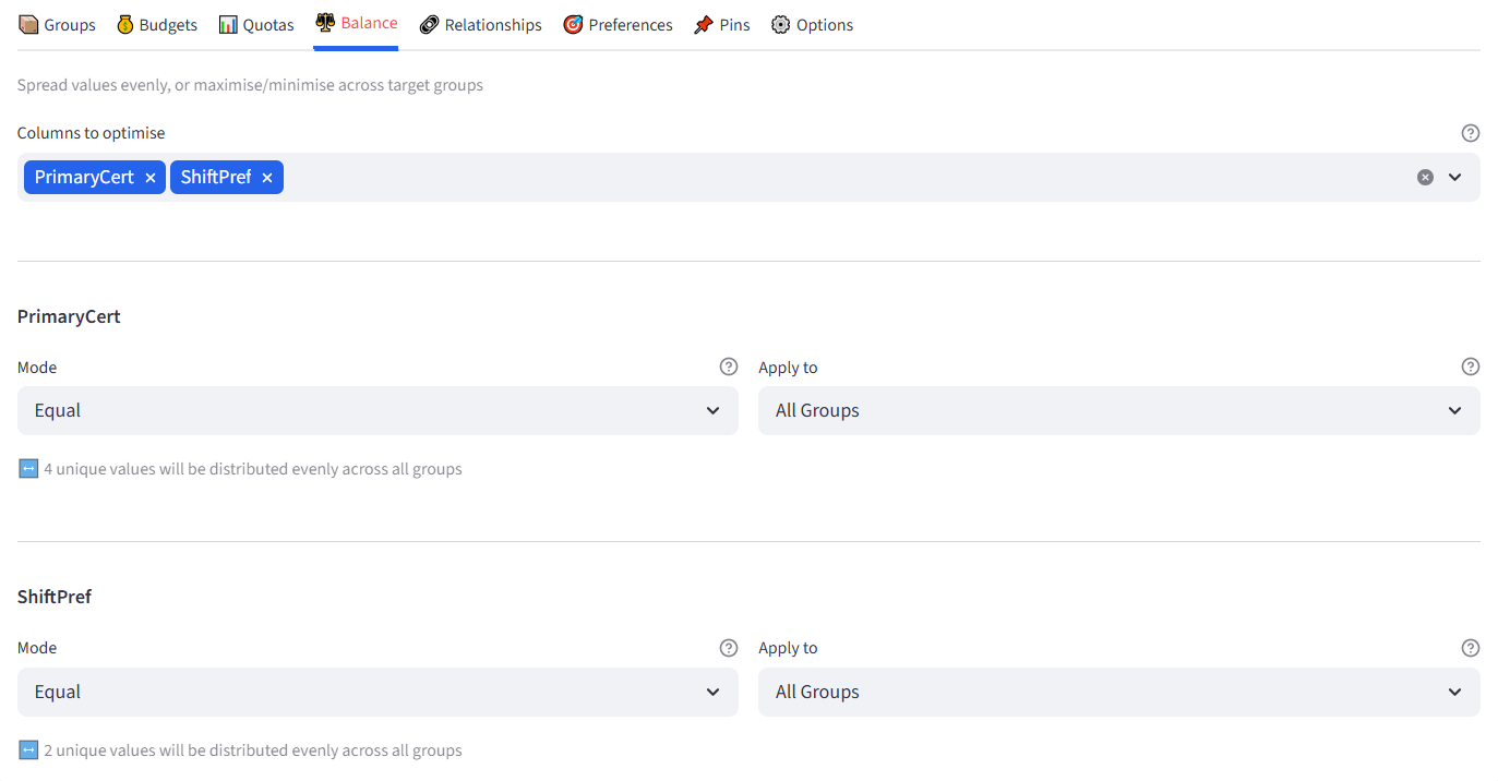
Step 8: Run & Validate

Click Run Optimizer.
Check: each line has 2–3 Level 3 operators, experience years are 30–55, primary certifications are spread, safety scores are in range.
Export for the floor supervisor.

Expected Outcome

Each line has 5–7 operators with 2–3 Level 3 certified. Experience years per line fall between 30–55. Primary certifications (CNC, Welding, Assembly, Quality) are spread evenly. Shift preferences are balanced. Safety scores are within the specified range.

This configuration ensures no line is understaffed on key certifications and no line is loaded with all inexperienced operators. Save the rules and reuse them quarterly when operators rotate.

This example uses 24 operators across 4 lines. Factories with 80–200 operators across 8–12 lines and multiple shift patterns use the same approach. Increase the solver timeout for larger workforces.

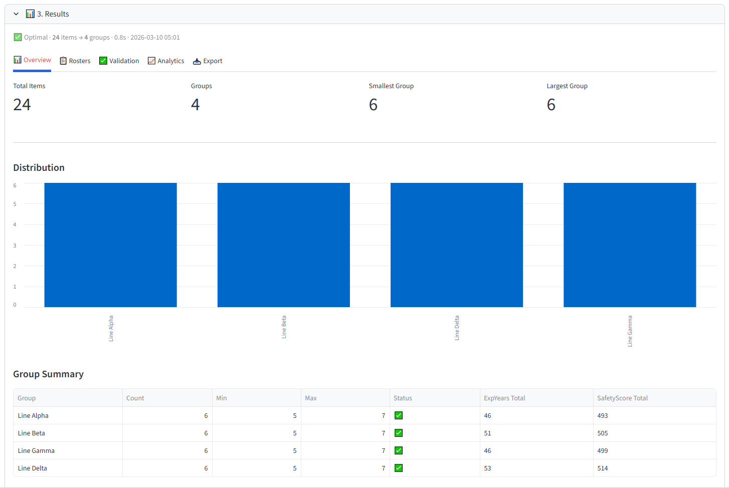
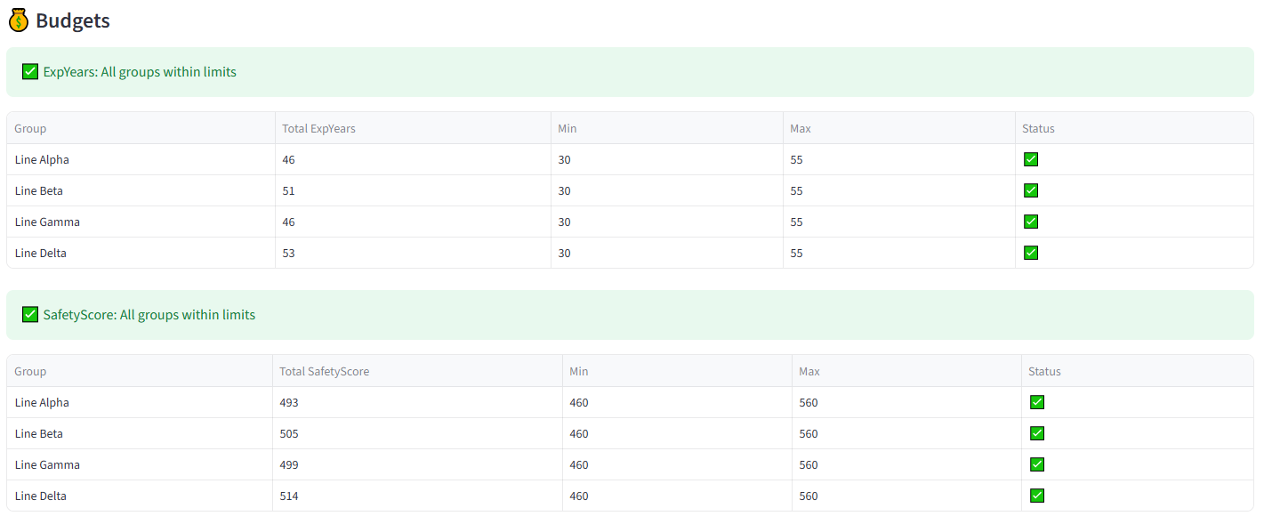
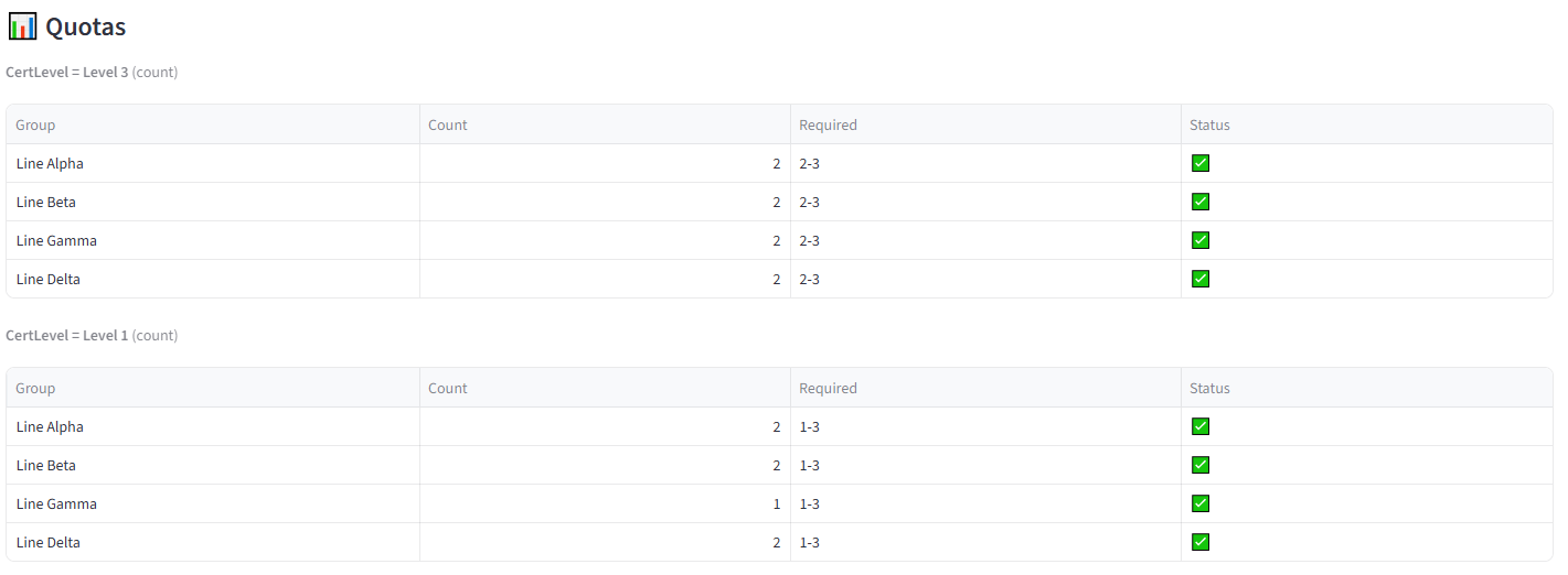
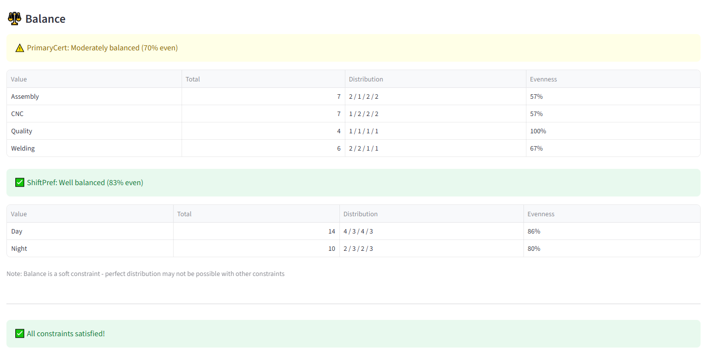
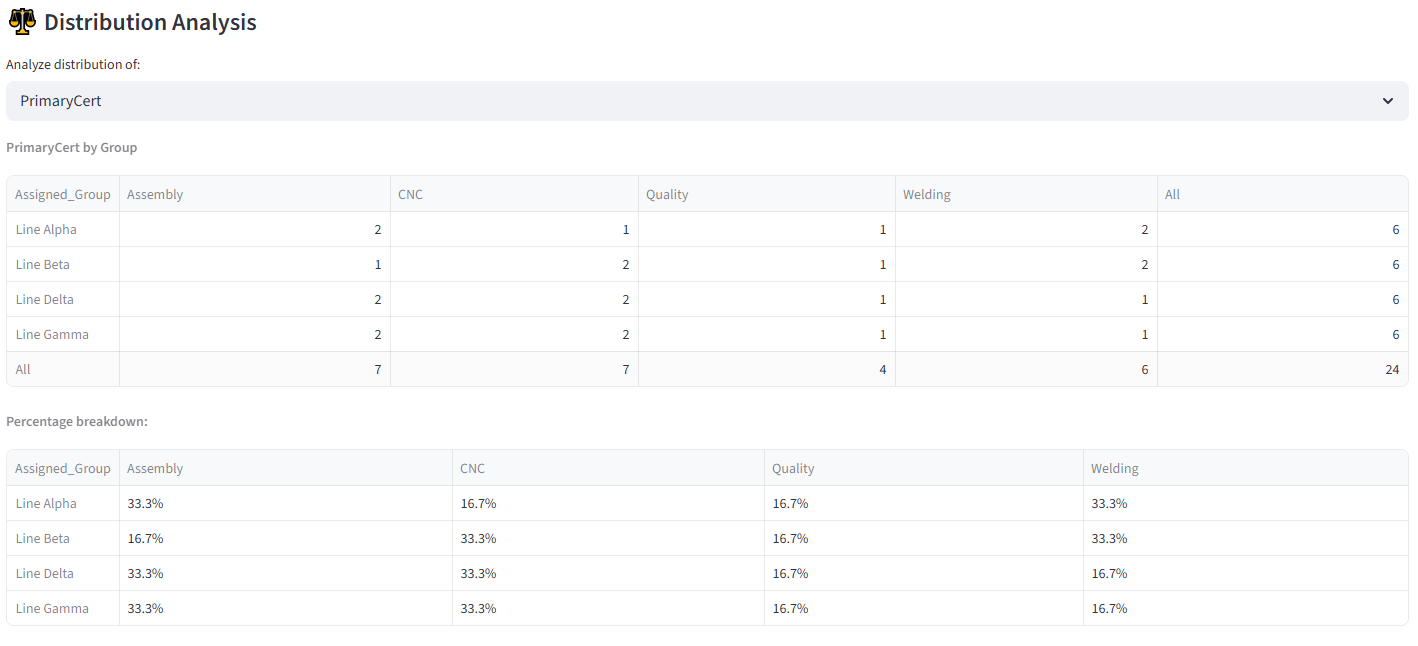
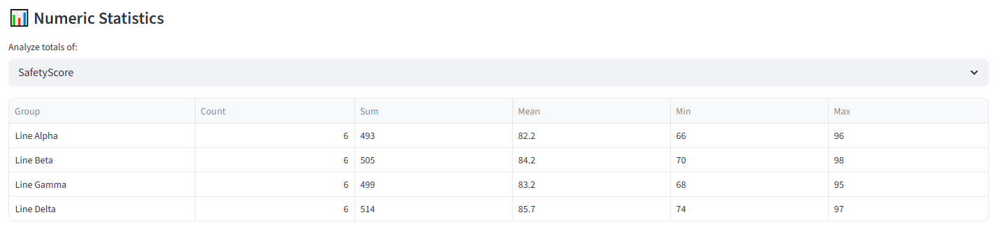
Appendix I: Procurement — Vendor Panel Selection

Scenario

Main Roads is forming an 10-vendor panel from 30 tender responses across four service categories: Civil, Electrical, Mechanical, and Environmental. The procurement team must select the strongest vendors while satisfying government procurement policy: Indigenous supplier representation, regional coverage, category coverage, a cap on any single region’s dominance, and a total estimated contract value ceiling.

The top 10 vendors by capability score are all based in Metro Perth, with no Indigenous-owned businesses. Selecting on merit alone violates three policy requirements. The solver finds the highest-scoring compliant panel automatically.

This demonstrates the select/reject pattern applied to procurement: 10 vendors are selected into the Panel group, and the remaining 20 go into Unsuccessful. The solver maximises capability scores in the Panel group while enforcing all policy constraints.

The data includes 30 vendors with service category, region, capability score (0–100 from the evaluation), risk score, estimated contract value, Indigenous ownership status, regional status, and whether the vendor was on the previous panel.

The Data

Save the following as vendor_panel.csv:

24 rows, 9 columns. First 5 rows shown:

Region	CapabilityScore	RiskScore	EstContractValue	Indigenous	Regional	PreviousPanel
Metro Perth	92	15	1800000	No	No	Yes
Pilbara	78	25	1400000	Yes	Yes	No
South West	85	18	1600000	No	Yes	Yes
Metro Perth	94	10	1500000	No	No	Yes
Metro Perth	88	20	1350000	No	No	Yes

Full CSV file: vendor_panel.csv

Step-by-Step Instructions

Step 1: Upload & Map

Upload vendor_panel.csv.
Set Unique ID to VendorID, Display Name to Company.
Import all columns.

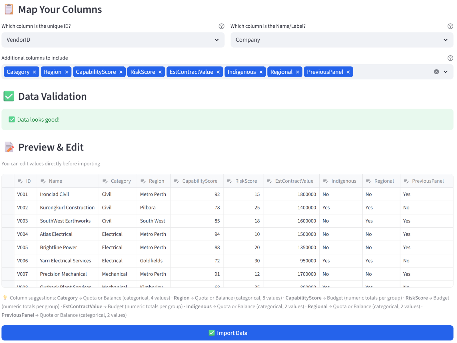
Step 2: Set Terminology

In the sidebar, expand Terminology.
Change Item to ‘Vendor’, Group to ‘Outcome’, ID to ‘Vendor ID’. Click Apply.

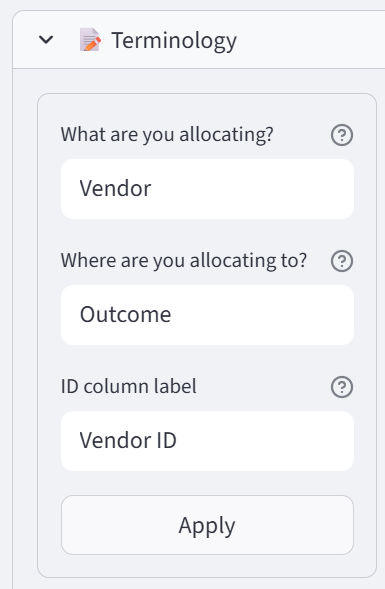
Step 3: Configure Groups – Successful vs Unsuccessful

Set Number of Outcomes to 2.
Rename: Panel, Unsuccessful.
Set Panel to Min 10 / Max 10 (exactly 10 vendors).
Set Unsuccessful to Min 20 / Max 20.

Tip: This is the select/reject pattern. The solver picks the best 10 that satisfy all policy constraints. The remaining 20 go into Unsuccessful.

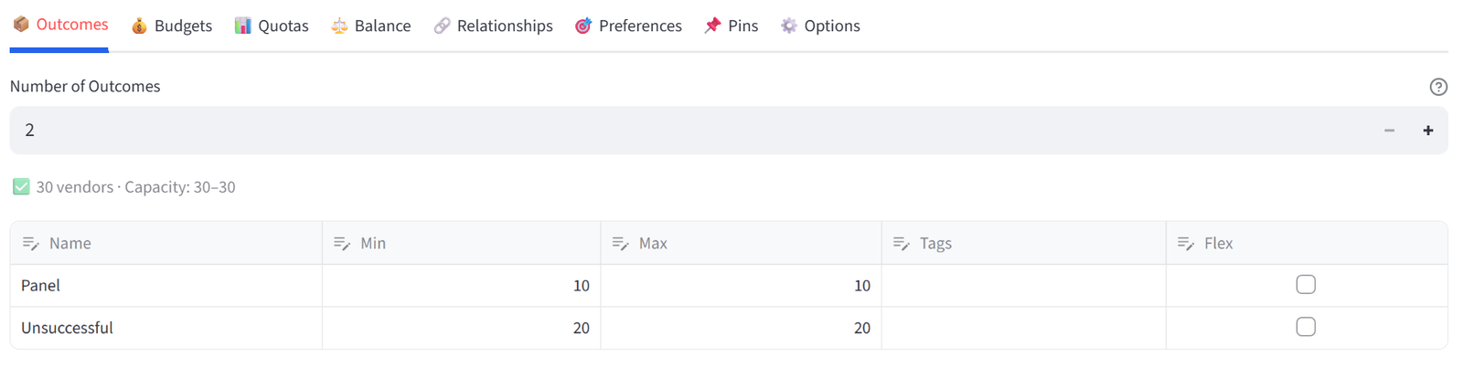
Step 4: Set Balance — Maximise Capacity

Go to the Balance tab.
Select CapabilityScore from the multiselect.
Set Mode to Maximise. Set Target group to Panel.

Tip: The solver will try to place the highest-scoring vendors into the Panel. But the policy quotas and budget below will override pure merit where needed — and the tool documents exactly where and why.

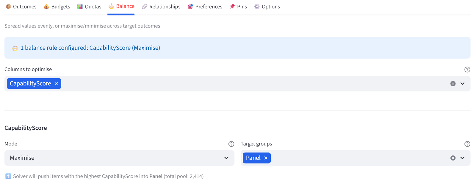
Step 5: Set Budget — Total Contract Value Cap

Go to Budgets tab. Select EstContractValue.
Set Panel: Min Total to 0, Max Total to 12000000.
Set Unsuccessful: increase Max to be unconstrained (Min 0, Max 99999999).

Tip: The $12M contract value ceiling means the solver cannot simply select the 10 largest vendors. The top 10 by score alone total $15.25M — over budget. The solver must trade off some high-value vendors for smaller ones to stay within the cap.

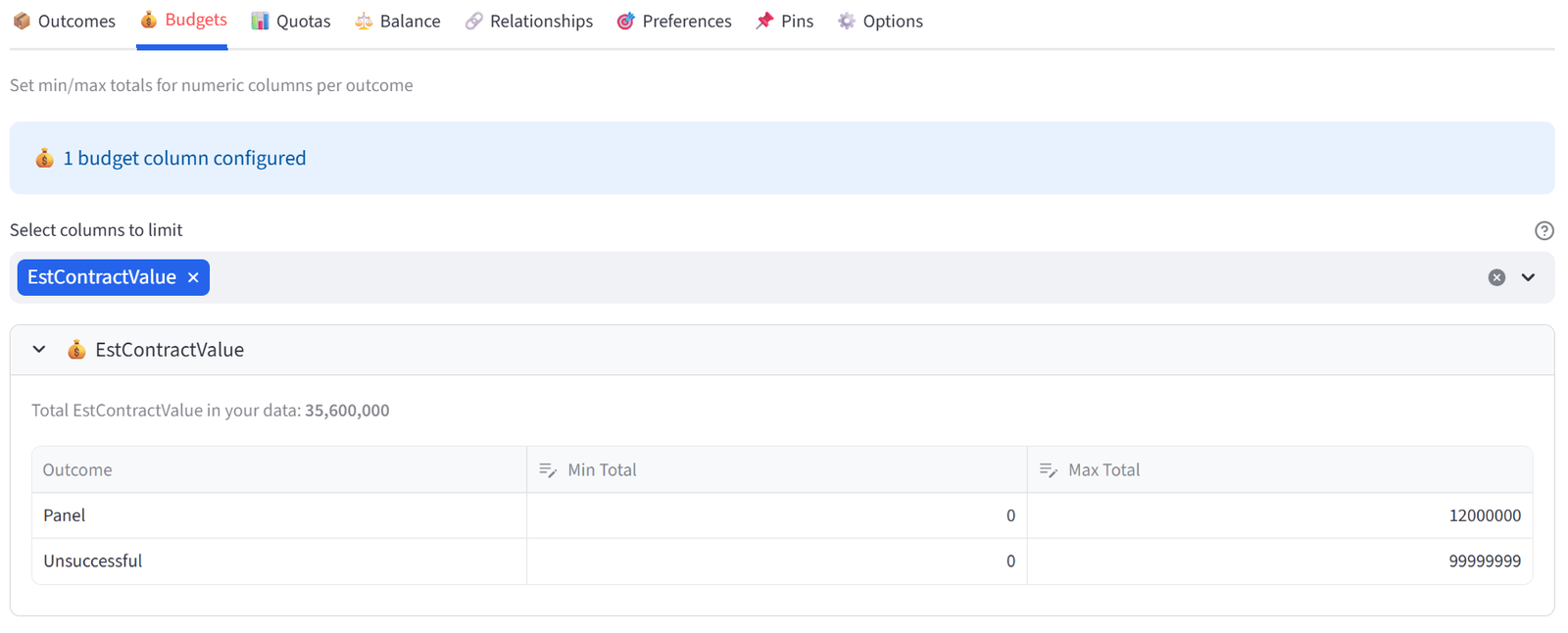
Step 6: Set Quotas — Indigenous Representation

Go to Quotas tab. Use Count mode.
Column: Indigenous, Value: Yes, Min: 2, Max: 10. Apply to: Panel. Click Add.

Tip: At least 2 of the 10 panel members must be Indigenous-owned businesses. There are 8 Indigenous vendors in the pool. The max of 10 means there is no upper cap — if merit supports more, the solver can include more.

Step 7: Set Quotas — Regional Representation

Stay on Quotas tab.
Column: Regional, Value: Yes, Min: 2, Max: 10. Apply to: Panel. Click Add.

Tip: At least 2 regional vendors. There are 16 regional vendors in the pool, so this is easily achievable.

Step 8: Set Quotas — Category Coverage

Stay on Quotas tab.
Under Quick rule: require at least one of every value, select Column: Category, Apply to: Panel. Click Add.

Tip: Every service category must be represented on the panel. This quick rule defaults to 1-9999 ensuring at least one of each Category is selected. Total minimums (1+1+1+1=4) leave room for the solver to optimise the remaining places on merit.

Step 9: Set Quotas — Regional Concentration Cap

Stay on Quotas tab.
Column: Region, Value: Metro Perth, Min: 0, Max: 5. Group: Panel. Click Add.

Tip: No more than 5 of the 10 panel members can be from Metro Perth. Without this constraint, all 10 would be Metro Perth (the highest-scoring vendors are all there). This forces geographic diversity.

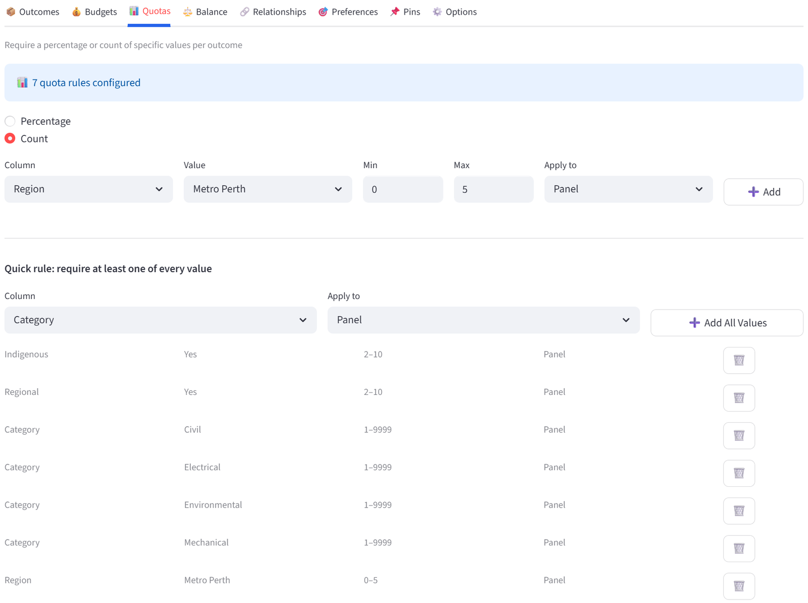
Step 10: Run & Validate

Click Run Optimizer.
Check Validation: Panel has exactly 10 vendors, at least 2 Indigenous, at least 2 regional, all 4 categories covered, no more than 5 from Metro Perth, total contract value ≤ $12M.
Review the Rosters tab: the Panel group should contain the highest-scoring vendors that satisfy all policy constraints.
Compare the average CapabilityScore in Panel vs Unsuccessful — there should be a clear gap.
Export the Panel list for the evaluation committee and the Excel report for the probity file.

Expected Outcome

The Panel contains 10 vendors with an average capability score of approximately 80–85. The Unsuccessful group averages lower. Total estimated contract value is at or below $12M.

At least 2 Indigenous-owned vendors are included. At least 2 regional vendors are on the panel. All 4 service categories are represented. Metro Perth is capped at 5, forcing the inclusion of vendors from the Pilbara, South West, Great Southern, or Goldfields.

Some high-scoring Metro Perth vendors will miss out — for example, one of Brightline Power (88), UrbanEdge Civil (88), or Core Electrical Solutions (86) may be displaced by a lower-scoring regional or Indigenous vendor to satisfy policy requirements. The tool documents exactly which constraint caused each trade-off.

This is the select/reject pattern applied to procurement. The solver maximises capability in the Panel group while enforcing every policy constraint. The Unsuccessful group is the reject pool. The Excel export includes a Constraints sheet listing every rule as a complete audit trail — attach it to the probity report.

This example uses 30 vendors for 10 panel places. The same approach scales to 200+ tender responses for panels of any size. Save the rules and reuse them for future panel refreshes with a new evaluation register.